Why Alarm Overload Is a Hidden Industrial Safety Risk

A control room operator watches a screen light up with dozens of alarms in under a minute.

Most are low-priority. A few are duplicates. One, buried somewhere in the middle of the list, is the early signal of a process upset that could escalate into a real incident. By the time it’s acknowledged, the window to act has narrowed considerably.

This scenario has a name in industrial automation circles: alarm overload, sometimes called alarm flooding.

It’s one of the most underrated risks in process safety, not because it’s rare, but because it hides in plain sight.

Alarms are supposed to protect operators and equipment. When there are too many of them, they do the opposite.

This article breaks down what alarm overload actually is, why it develops in well-intentioned control systems, the safety and financial consequences it creates, and the practical steps used to fix it, grounded in the ISA-18.2 / IEC 62682 alarm management standard that most modern facilities are measured against.

What Is Alarm Overload?

Alarm overload occurs when the number of alarms presented to an operator exceeds what a person can realistically process, prioritize, and respond to during a given period. It’s a human factors problem wearing an engineering disguise.

Industry benchmarks from the Engineering Equipment and Materials Users’ Association (EEMUA 191) and ISA-18.2 define manageable alarm rates for a single operator:

  • Steady-state operation: no more than roughly 1 alarm every 10 minutes on average
  • During a plant upset: a well-managed system should avoid more than about 10 alarms in the first 10 minutes following a major disturbance

In practice, many facilities blow past these numbers by an order of magnitude. Some documented upset conditions have produced hundreds of alarms in the first few minutes far beyond what any single person can meaningfully triage.

Why Alarm Overload Happens

Alarm overload is rarely the result of one bad decision. It accumulates gradually, often through years of well-meaning engineering additions.

Poorly Set Alarm Thresholds

Setpoints copied from generic vendor defaults, rather than tuned to actual process behavior, tend to trigger far more often than necessary.

A pressure alarm set too close to normal operating variance will fire constantly, even when nothing is actually wrong.

Alarm Duplication Across Systems

Modern plants often layer a DCS, a PLC-based safety system, and a separate SCADA or building management layer.

When the same physical condition triggers alarms in more than one of these systems, the operator sees redundant alerts that add noise without adding information.

Chattering and Fleeting Alarms

An alarm that repeatedly activates and clears within seconds, often due to signal noise or a setpoint sitting too close to a fluctuating process value, is called a “chattering” alarm. A single unstable measurement can generate dozens of alarm events in minutes.

No Formal Alarm Rationalization Process

Many facilities add alarms as instrumentation is installed but rarely remove or consolidate them later.

Without a structured rationalization process, the alarm database grows continuously and never gets pruned.

Consequence: Alarms Instead of Root-Cause Alarms

When a single root-cause event (like a pump trip) cascades into alarms on every downstream variable it affects, the operator is shown a dozen symptoms instead of one clear cause, a pattern known as an alarm flood.

The Hidden Safety Risk: Alarm Fatigue

The core danger of alarm overload isn’t the alarms themselves. It’s what they do to human attention over time. This phenomenon is known as alarm fatigue, and it shows up in a few predictable ways.

Desensitization

Operators begin to mentally filter out alarms as background noise, especially when the majority of past alarms turned out to be nuisance events.

Delayed response

With dozens of alarms competing for attention, genuinely urgent ones take longer to be identified and acted on.

Alarm shelving without review

Under pressure, operators may silence or acknowledge alarms in bulk just to clear the screen, sometimes bypassing the analysis that the alarm was meant to prompt.

Missed critical alarms entirely

In a true flood condition, a high-priority alarm can scroll off screen or get lost among dozens of lower-priority ones before it’s ever seen.

Alarm fatigue has been formally cited as a contributing factor in major industrial incidents, including well-documented refinery and chemical plant accidents where operators were presented with hundreds of alarms in the minutes before an escalation, making it effectively impossible to identify the one signal that mattered.

The uncomfortable truth is that a poorly managed alarm system can make a plant less safe than a bare-bones one because it trains operators through sheer repetition to treat alarms as routine rather than actionable.

Why This Risk Stays Hidden

Alarm overload rarely shows up as a line item in a safety audit the way a missing guardrail or an unlabeled valve would. It hides for a few structural reasons.

It doesn’t look broken

Every alarm is technically “working.” It’s firing when its condition is met. The system passes a functional test even while it’s operationally unusable.

It’s normalized gradually

Because the alarm count grows slowly over years, operators adapt incrementally and rarely flag it as a crisis until an incident forces the question.

Metrics aren’t tracked

Many facilities don’t monitor alarm rate, alarm priority distribution, or standing alarm counts at all, so there’s no data trail showing the problem exists.

Responsibility is diffused

Alarms are added by process engineers, instrumentation techs, and control system integrators over time. No single person owns the alarm system as a whole.

How to Fix Alarm Overload

Alarm Rationalization

This is the foundational fix defined in ISA-18.2. Every existing alarm is reviewed against a documented set of criteria: does it have a clear cause, a clear consequence if ignored, and a clear operator action? Alarms that fail this test are removed, combined, or reclassified as informational messages rather than alarms.

Prioritization by Consequence and Time-to-Respond

Alarms should be tiered (commonly Priority 1–3 or Critical/High/Low) based on the severity of the consequence and how much time the operator realistically has to respond.

Not every deviation deserves the same visual and audible treatment as an emergency shutdown condition.

Deadbanding and Time Delays

Adding a deadband (a buffer zone around the setpoint) or a short time delay before an alarm activates can eliminate the majority of chattering alarms without weakening genuine detection.

Alarm Flood Suppression Logic

Modern alarm management software can automatically suppress downstream “consequence” alarms when a known root-cause alarm has already activated, so operators see one clear signal instead of a cascade of symptoms.

Ongoing Alarm Performance Monitoring

Tracking metrics like average alarms per hour, top 10 most frequent alarms, and standing alarm counts turns alarm management from a one-time project into a maintained discipline.

Facilities that revisit this data quarterly catch new nuisance alarms before they accumulate into another flood.

Operator Involvement in Design

Operators are the end users of the alarm system, and their input on which alerts are genuinely actionable is often more accurate than theoretical risk models alone.

Alarm Overload vs. Alarm Rationalization: Quick Comparison

AspectAlarm Overload (Unmanaged)After Rationalization
Alarms per 10 min (steady state)Often 5–20+Target: ~1
Alarm priority structureFlat or inconsistentTiered by consequence/urgency
Root-cause visibilityBuried in symptom alarmsIsolated and highlighted
Operator response accuracyDegrades under loadMaintained under upset conditions
Nuisance/chattering alarmsCommon, untrackedSuppressed or eliminated
OwnershipDiffused across teamsAssigned, documented process

Frequently Asked Questions

What is considered a manageable alarm rate for an operator?

Industry guidance (EEMUA 191 / ISA-18.2) generally targets no more than about one alarm every 10 minutes during steady-state operation, and no more than roughly 10 alarms in the first 10 minutes following a major process upset.

What’s the difference between alarm overload and an alarm flood?

Alarm overload is the broader, chronic condition of a system generating more alarms than an operator can reasonably manage.

An alarm flood is a specific, acute event, typically triggered by a process upset, where a large burst of alarms activates in a short window.

Can alarm overload really cause an accident?

Yes. Alarm fatigue from chronic overload has been identified as a contributing factor in several major industrial incidents, where operators were unable to identify the critical alarm among hundreds of simultaneous alerts.

How often should an alarm system be reviewed?

Best practice under ISA-18.2 calls for periodic alarm performance reviews (often quarterly) plus a full rationalization exercise whenever the process, instrumentation, or control system undergoes significant change.

Is alarm overload only a problem in large refineries and chemical plants?

No. Any facility with a DCS, PLC-based control system, or building automation platform, including manufacturing plants, water treatment facilities, and commercial BMS installations, can develop alarm overload as instrumentation and control points accumulate over time.

Final Thoughts

Alarm overload doesn’t announce itself the way a mechanical failure or a safety breach does.

It builds quietly, alarm by alarm, until the system meant to protect operators has become something they’ve learned to tune out.

The fix isn’t more alarms or louder ones. It’s fewer, better-prioritized alarms that operators can actually trust and act on.

Facilities that treat alarm management as an ongoing discipline, rather than a one-time cleanup, tend to catch nuisance conditions before they compound into another flood and keep the alarm system doing the one job it exists for: getting the right signal to the right person in time to act.

What is a Fail-Safe System in Automation?

Industrial automation systems require increasing levels of operational dependability and safety.

Modern systems feature sophisticated equipment with mechanical, electrical, and thermal hazards.

Engineers have to simultaneously safeguard production continuity, equipment, and personnel. 

Engineers must protect personnel, equipment, and production continuity simultaneously. Conventional control strategies alone cannot guarantee acceptable risk reduction. For this reason, protective mechanisms are integrated into automation architectures. 

Among these mechanisms, fail-safe systems hold critical importance. They ensure predictable behavior when faults or abnormal conditions occur.
Instead of maximizing productivity during failure, they prioritize safety outcomes. 

Their design philosophy assumes that components can and will fail. Understanding fail-safe principles is essential for responsible automation engineering practice.
This article reviews the concept of fail-safe systems, their design philosophy, architectural principles, standards compliance, and practical industrial applications.

Fundamentals of Automation Control Systems

Industrial automation relies on deterministic control executed by programmable devices. Controllers receive input signals from sensors distributed across machinery. These inputs represent temperature, pressure, position, or safety status.

The controller processes signals using predefined logical algorithms. Outputs then command actuators such as motors, valves, and contactors. Standard control systems emphasize efficiency, availability, and productivity optimization.

They are widely deployed in manufacturing. Also, they are utilized in water treatment sectors and energy facilities.

Vendors such as Siemens and Rockwell Automation provide global automation platforms. These systems typically focus on maintaining continuous process operation.

However, continuous operation is not always the safest outcome. When abnormal conditions arise, protective intervention becomes necessary.
Fail-safe systems address this requirement by ensuring controlled shutdown. They complement standard control layers within hierarchical automation architectures.

What is a Fail-Safe System in Automation?

A fail-safe system is engineered to default to a safe state. This transition occurs automatically when a fault is detected.

The safe state minimizes risk to humans and equipment. Unlike conventional systems, performance during failure is not prioritized.

Instead, predictable hazard mitigation becomes the primary objective. A fail-safe design anticipates power loss and component malfunction. Outputs are typically de-energized to eliminate hazardous motion. 

For example, a motor contactor may drop out during failure. This prevents unintended mechanical movement or energy release. The principle applies across electrical, mechanical, and software domains. 

Fail-safe systems are foundational elements of functional safety engineering. They contain and manage faults to prevent large-scale failure events.

Relationship with Functional Safety Standards

Fail-safe design principles align closely with international safety standards. The most recognized standard is IEC 61508 for electrical safety systems. Another widely applied machinery standard is ISO 13849.

These standards define systematic processes for achieving risk reduction. They introduce measurable integrity metrics for safety functions. Designers must demonstrate that the dangerous failure probability remains acceptable.

Compliance requires structured lifecycle documentation and verification. Hardware architecture must tolerate predictable fault conditions. Software development must follow validated and traceable methodologies.

Fail-safe systems are therefore not arbitrary protective additions. They are carefully engineered to meet defined performance levels. Certification provides confidence in their reliability under hazardous scenarios.

Core Design Philosophy of Fail-Safe Systems

The fundamental philosophy assumes that failures are inevitable. Therefore, systems must respond safely rather than unpredictably. This mindset differs significantly from traditional reliability engineering.

Reliability seeks uninterrupted performance under normal conditions. Fail-safe engineering focuses on controlled behavior during abnormal conditions. Designers intentionally define what “safe” means for each application.

In many electrical systems, the safe state is de-energization. Springs may return mechanical components to neutral positions. Valves may close automatically when control pressure disappears.

Electrical circuits often employ normally closed safety contacts. If wiring breaks, the circuit opens and stops operation.

This arrangement ensures the detection of disconnection faults. Such design practices reduce the likelihood of hidden, dangerous failures. Predictable shutdown becomes a deliberate and verified outcome.

Architectural Principles and Redundancy

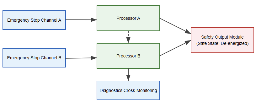
Redundancy is frequently integrated within fail-safe architectures. Dual-channel circuits monitor safety devices independently. Both channels must agree before hazardous motion is permitted.

If disagreement occurs, the system initiates a shutdown. This structure reduces vulnerability to single-component failure. Some systems implement diverse processor architectures for added robustness.

Safety controllers often compare execution results cyclically. Memory integrity checks are performed during each scan cycle.

Input circuits detect short circuits and cross faults. Output circuits may monitor feedback from external relays. 

These mechanisms collectively increase diagnostic coverage significantly.
Architectural discipline distinguishes fail-safe systems from conventional controls. The objective remains minimizing undetected dangerous faults.

What is a Fail-Safe System in Automation?

Basic Fail-Safe Architecture with Redundant Channels and Safe-State Output

Electrical Implementation Techniques

Electrical fail-safe design uses specific circuit arrangements. Emergency stop circuits commonly utilize normally closed pushbuttons. Pressing the button opens the safety circuit deliberately. If wiring breaks, the circuit also opens automatically. 

This behavior ensures detection of cable disconnection failures. Safety relays incorporate force-guided contact mechanisms internally. These contacts mechanically prevent contradictory output states. 

Redundant contactors may disconnect motor power independently. Feedback loops confirm actual de-energization of power circuits. Power supplies supporting safety systems often include redundancy. 

Loss of one supply does not immediately compromise integrity. Ground fault monitoring may also be incorporated for detection. These techniques collectively enhance electrical hazard mitigation capability.

Software Considerations in Fail-Safe Logic

Software plays a critical role in modern fail-safe systems. Safety logic must execute deterministically within bounded cycle times. Watchdog timers supervise execution to detect software freeze conditions.

If timing limits are exceeded, the system transitions safely. Programming environments may restrict unsafe coding constructs intentionally.

Certified safety function blocks are commonly utilized. These blocks undergo extensive verification before release. 

User modifications are controlled through structured change management. Traceability from requirement to implementation is mandatory.

Documentation supports later audits and regulatory inspections. Fail-safe software, therefore, complements hardware redundancy measures. Both domains cooperate to achieve acceptable risk reduction.

Communication and Network Reliability

Distributed automation increasingly relies on network communication. Fail-safe systems must maintain integrity across communication channels.

Safety protocols add redundancy and validation mechanisms. Time stamping and sequence counters detect transmission anomalies. 

Corrupted or delayed messages trigger protective responses. Deterministic fault detection timing remains essential for compliance. Network configuration changes may require revalidation of safety analysis.

Safety communication layers ensure consistent behavior across devices. They support complex machines with multiple protective zones.

Robust communication design prevents hidden faults within networks. This ensures coordinated and predictable protective action.

Industrial Applications of Fail-Safe Systems

Fail-safe systems are widely deployed across industries. Automotive production lines utilize protective guarding and interlocks. Robotic cells immediately halt when light curtains detect intrusion.

Process industries apply fail-safe valves in hazardous environments. Companies such as Honeywell provide integrated safety platforms.

Oil and gas facilities often demand high-integrity shutdown systems. Boiler management systems rely on flame failure detection circuits.

Conveyor systems implement safe speed monitoring functions. Elevators employ fail-safe braking mechanisms for passenger protection.

In each scenario, a controlled shutdown protects human life. The cost of failure far exceeds equipment replacement expenses.

Economic and Strategic Considerations

Fail-safe systems generally increase project capital expenditure. Redundant components and certification processes require investment. Engineering expertise must support validation and documentation activities.

However, accident consequences often involve severe financial loss. Noncompliance can result in severe regulatory sanctions and legal consequences.

Insurance frameworks frequently mandate certified protective systems. Reputation damage following incidents may be irreversible.

Strategic planning, therefore, incorporates safety from the initial design stages. A layered architecture often separates control and safety domains. Standard controllers manage production efficiency and optimization. 

Dedicated safety systems oversee the management of hazardous energy sources. This structured separation enhances clarity and compliance.

Long-term operational sustainability depends upon responsible safety investment.

Integration with Safety PLC Technology

Modern fail-safe implementations frequently use specialized controllers. These devices are known as Safety PLC units.

They differ from conventional controllers through redundancy and diagnostics. Dual processors compare logic execution results continuously.

Certified programming environments restrict unsafe implementation practices. Safety Integrity Levels define measurable performance expectations.

If internal inconsistencies arise, outputs transition automatically. This ensures predictable behavior during internal faults.

Safety PLCs, therefore, embody fail-safe principles systematically. They integrate hardware, software, and diagnostics coherently. Such integration simplifies compliance within complex automation systems.

Conclusion

This article introduced the principles of fail-safe systems within industrial automation environments.

It explained how a fail-safe design prioritizes predictable safe behavior during faults. Architectural redundancy and diagnostic coverage were described thoroughly.

International standards define measurable integrity requirements for implementation. Electrical and software techniques cooperate to enforce protective shutdown.
Industrial applications demonstrate their necessity across hazardous operations. 

Economic analysis confirms that prevention outweighs accident consequences.
Fail-safe philosophy assumes failure yet controls its impact responsibly. Integration with approved controllers improves dependability and compliance. 

Knowing these ideas helps engineers to create automation systems that properly safeguard people, machinery, and long-term operating continuity.

FAQs: What is a Fail-Safe System in Automation?

What is a Fail-Safe System in Automation?

Upon failure, a system sets to default to a secure condition. 

Automation benefits from fail-safe systems since they provide 

During power outages or fault conditions, they help to stop dangerous situations from worsening. 

What kind of arrangement is a fail-safe circuit looking for to identify wiring problems? 

It uses normally closed contacts that open when wiring integrity is compromised.

Are fail-safe systems required by standards?

Yes, standards like IEC 61508 require validated safety behavior. This is also applicable for standards like ISO 13849.

Do fail-safe systems reduce productivity?

They may interrupt operation, but they significantly reduce catastrophic risk.

Three Types of Starter Motor

In internal combustion engine systems, the starter motor is a crucial device. It is responsible for initiating engine operation by cranking the crankshaft. The action persists until the engine can maintain combustion on its own.

Despite being frequently underestimated, the starter motor must generate high torque rapidly. It must also operate reliably under harsh electrical and thermal conditions.

Furthermore, under severe mechanical circumstances. Several starter motor designs have been developed. 

These designs aim to improve efficiency and reduce size. Furthermore, dealing with enhancing durability. Knowledge of different starter motor types is critical.

This knowledge benefits engineers involved in automotive, industrial, or power systems. Furthermore, it is useful for technicians and students of the equivalent areas.

This article explains three common types of starter motors. It covers their construction and working principles.

Furthermore, it deals with advantages and limitations. Finally, it mentions the typical applications.

Before discussing specific types, it is useful to pause. Understanding the basic operation of a starter motor provides the necessary foundation.

To supply electrical energy, the ignition switch is initially turned to the START position. The latter comes from the battery and flows to the starter solenoid.

The solenoid performs two key functions. First, it is to ensure engagement of the starter pinion gear and engine flywheel.

It also closes a high-current circuit to power the motor. The motor then produces high torque at low speed. 

The flywheel and crankshaft then start to rotate. Once the engine starts, the starter is disengaged to prevent damage caused by overspeed.

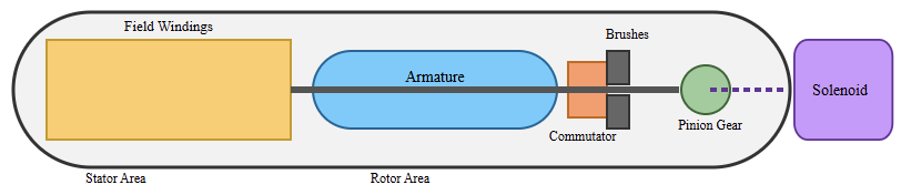
The following figure indicates a basic starter motor system showing the battery, ignition switch, and solenoid. Furthermore, it illustrates the pinion gear, flywheel, and engine crankshaft.

Direct Drive Starter Motor

Construction and Design

The direct drive starter motor is the oldest and simplest starter motor design.
The primary distinction lies in the direct engagement of the motor shaft with the pinion gear. There is no intermediate gear reduction.

The armature, field windings (or permanent magnets), commutator, and brushes are housed together.

The robust cylindrical casing is used to enclose them. The pinion gear is mounted on the armature shaft. 

It is engaged with the flywheel via a solenoid-operated mechanism. Because there is no gear reduction, the motor itself must be relatively large. It must also be powerful to produce the required high torque. 

This torque is needed to crank the engine directly. The next figure depicts a cross-sectional diagram of a direct drive starter motor. It shows the armature, field windings, brushes, solenoid, and pinion gear.

Working Principle

The ignition key is turned to the START position to enable current to flow through the solenoid.

Then the solenoid pushes the pinion gear into mesh with the flywheel. High current flows through the motor windings simultaneously. This creates a strong magnetic field.

When the magnetic field interacts with armature conductors, torque is produced. The armature rotates at a relatively low speed. Nevertheless, high torque is produced, which turns the engine flywheel. 

The ignition key is released as soon as the engine starts and the solenoid de-energizes. The pinion gear then disengages from the flywheel.

Advantages

Direct drive starter motors have a simple and rugged construction. Their mechanical simplicity makes them relatively straightforward to manufacture and repair. They are also highly durable. 

They can tolerate harsh operating conditions. This may include high temperatures and vibration.

For many years, they were the standard choice. This was especially true in older vehicles and industrial engines.

Limitations

The main disadvantage of direct drive starter motors is their size and weight. Because torque is produced directly by the motor without gearing, the motor must be large. It must also draw a very high current from the battery.

This results in greater electrical stress. The stress affects both the battery and the cables. Additionally, direct drive starters are generally less efficient. They perform worse compared to modern designs.

Typical Applications

Direct drive starter motors are commonly found in older vehicles. They are also used in heavy-duty machinery. In addition, they are applied in tractors and stationary engines.

They are still used in applications where simplicity and robustness are priorities. In these cases, compactness or efficiency is less important.

Gear Reduction Starter Motor

Construction and Design

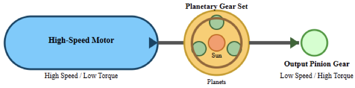
The starter motor with gear reduction is also known as a reduction gear starter. It incorporates a gear train between the motor shaft and the pinion gear. Typically, a small high-speed motor drives a set of reduction gears. 

These gears may include planetary gears. The gears increase torque while reducing output speed.

The motor itself is often smaller and lighter. It is lighter than the motor used in direct drive designs. Permanent magnets are frequently used instead of field windings. 

This further reduces size and improves efficiency. The upcoming figure indicates a diagram of a gear reduction starter motor showing a high-speed motor, a planetary gear set, and an output pinion gear.

Working Principle

When energized, the starter motor rotates at high speed. However, higher speed results in lower available torque.

The reduction gear train converts this high-speed, low-torque output. It becomes a low-speed, high-torque motion at the pinion gear.

This amplified torque is sufficient to crank the engine effectively. It works even under cold-start conditions.

The solenoid mechanism functions similarly to that of a direct drive starter. It engages the pinion gear with the flywheel. This step occurs before power is applied to the motor.

Advantages

Starter motors with gear reduction offer several significant advantages. They are lighter and more compact than direct drive starters.

This helps reduce overall vehicle weight. As mentioned above, these types of starter motors contain higher efficiency. They use less battery current as a result. 

At the same time, they deliver equal or greater cranking torque. This improves battery life. It also enhances cold-start performance. Another benefit is improved reliability.


Because the motor operates at a higher speed with lower torque stress, mechanical wear is reduced. This applies to internal components.

Limitations

The primary drawback of gear reduction starters is increased mechanical complexity. The inclusion of a gear train introduces additional components. These components can wear over time. 

Manufacturing costs are also slightly higher. They are higher compared to direct drive starters. However, modern materials and lubrication methods have minimized these concerns.

Typical Applications

Starter motors with gear reduction are widely used in modern passenger vehicles. They are also common in light trucks and motorcycles.

They are frequently used in hybrid vehicles. Small industrial engines also benefit from their efficiency and compactness.

Permanent Magnet Starter Motor

Construction and Design

The permanent magnet starter motor uses permanent magnets mounted on the stator. These replace traditional field windings; hence, there is no need for field coils. This effect leads to a reduction in weight, size, and electrical losses.

Permanent magnet starter motors are often combined with gear reduction mechanisms. However, they can also exist in direct drive configurations. The armature, commutator, brushes, solenoid, and pinion gear are similar. 

They resemble those found in other starter motor types. However, the magnetic field is provided entirely by permanent magnets.

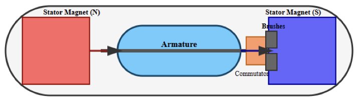
The figure below shows the internal layout of a permanent magnet starter motor, highlighting stator magnets, armature, and brush assembly.

Working Principle

When current flows through the armature windings, interaction occurs. It happens between the armature magnetic field and the fixed magnetic field.

This interaction produces torque. The fixed field comes from the permanent magnets.

Since the magnetic field does not rely on current flowing through field windings, efficiency improves. Electrical efficiency is therefore higher.

In many designs, the permanent magnet motor drives the pinion through a gear reduction system. This further increases torque output. At the same time, the motor remains compact.

Advantages

Permanent magnet starter motors are highly efficient and lightweight. The elimination of field windings reduces copper losses.

It also reduces heat generation. This allows for faster cranking speeds. It also improves cold-start performance.

Their compact size makes them ideal for modern vehicles. This is especially true where engine bay space is limited.

Another advantage is reduced current consumption. For this reason, the battery and charging systems experience less stress.

Limitations

Environmental conditions, such as high temperatures, affect starter motors. In this case, a permanent magnet is not an exception.

Mechanical shock can also impact these magnets. Excessive heat can weaken the magnets over time. Such damage reduces motor performance.

Additionally, permanent magnet starter motors may be less suitable for huge engines. Huge engines require extremely high torque. Magnet size and strength impose practical limits.

Typical Applications

Permanent magnet starter motors are commonly used in modern passenger cars. They are also found in compact vehicles and motorcycles.

They are popular in small engines as well. Examples include generators, lawn equipment, and light industrial machinery.

Comparison of the Three Starter Motor Types

Each starter motor type offers a different balance of performance factors. These include torque, efficiency, size, and durability.

While direct drive starters offer a simple and robust design, they tend to be heavy and inefficient.

Gear reduction starters provide higher efficiency and torque density. As a result, modern vehicles make them the preferred choice.

Permanent magnet starters further improve efficiency and compactness. This is especially true when combined with reduction gears.

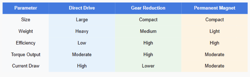
The following table shows a comparison between starter motors. It indicates size, weight, efficiency, torque output, and current draw for direct drive, gear reduction, and permanent magnet starter motors.

Conclusion: Types of Starter Motor

Reliable engine operation depends heavily on the starter motor. Their design has evolved significantly to meet modern demands. These demands include efficiency and performance.

The three main types include direct drive, gear reduction, and permanent magnet starter motors.

Each type has distinct construction features. Each also has unique operating principles and application areas.

Direct drive starters offer simplicity and durability. Gear reduction starters provide superior torque-to-size ratios. Permanent magnet starters deliver excellent efficiency and compactness.

By understanding these differences, engineers can make informed decisions. It is also applied to technicians as well as students.

These decisions apply to designing, selecting, or maintaining engine starting systems. This leads to an improvement in reliability, efficiency, and overall system performance.

FAQ: Types of Starter Motor

What are the main types of starter motors used in engines?

The main types include Direct Drive, Planetary/Gear Reduction, and Permanent Magnet starter motors.

Other variants, such as Permanent Magnet Direct Drive (PMDD) and Off-Set Gear Reduction (OSGR), also exist, but the three above are the most widely referenced. 

What is a Direct Drive starter motor?

A Direct Drive starter motor is a traditional design in which the motor shaft is directly coupled to the pinion gear without reduction gearing.

When energized, the solenoid pushes the pinion to engage the flywheel, causing the engine to crank. 

What is a gear-reduction starter motor?

A gear-reduction starter motor uses a high-speed, compact motor coupled to a set of reduction gears (often planetary gears). These gears increase torque while reducing current demand.

This results in a smaller, lighter starter with comparable or better cranking power than direct drive designs. 

What is a Permanent Magnet starter motor?

A Permanent Magnet starter motor replaces traditional field windings with permanent magnets in the stator. This reduces size and weight and typically improves electrical efficiency.

These can exist with or without reduction gears, but are commonly considered gear-reduced designs. 

What’s the difference between Direct Drive and Gear Reduction types?

Direct Drive

Motor output goes straight to the pinion gear; usually heavier and draws more current.

Gear Reduction

Uses gears (often planetary) to multiply torque while allowing a smaller, high-speed motor. Gear reduction starters are lighter, draw less current, and are more common in modern vehicles. 

Why do modern vehicles prefer gear reduction starters?

Gear Reduction starters are more compact and efficient. They produce high torque with less current draw than direct drive starters.

This makes them suitable for vehicles with limited engine bay space and smaller batteries. 

Are permanent magnet starter motors more efficient?

Yes. Because permanent magnet starters use magnets instead of field windings to produce the magnetic field, they reduce electrical losses and heat generation.

This makes them generally more efficient and lighter than similar wound-field designs.

How to Tune a PID Controller

PID stands for Proportional–Integral–Derivative, and remains the most widely used control algorithm in the global industry.

They are mainly used in industrial automation and robotics. Also, in areas such as power electronics and process control. 

Their popularity comes from a good balance between simplicity and robustness. Plus, the performance they offer.

They possess a very simple structure. However, correctly tuning PID controllers can be a big challenge. Poor tuning may result in excessive overshoot. 

It may cause slow response, oscillations, or even instability. On the other hand, a well-tuned PID controller can significantly improve system performance. It can reduce energy consumption and extend equipment life. 

Fundamentals of PID control are explained in the present article. It provides practical, step-by-step guidance on how to tune a PID controller. Both classical and modern methods are covered.

Understanding the PID Controller

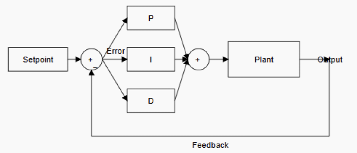
A PID controller generates a control signal based on the error (E). The error is between the desired setpoint and the actual measured output.

The output belongs to a system. The error signal is processed through three distinct terms. 

These terms are proportional, integral, and derivative. Each term contributes differently to the controller’s behavior.

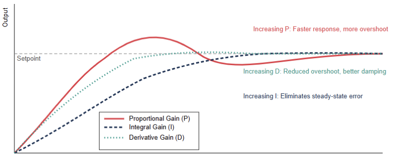
The proportional (P) term produces an output proportional to the current error. Increasing the proportional gain generally makes the system respond faster. Too much gain can cause oscillations or instability. 

The integral (I) term accumulates past errors over time. This term is responsible for eliminating steady-state error.

Excessive integral action can lead to slow response. It can also cause oscillatory behavior known as integral windup. 

The derivative (D) term predicts future error based on the rate of change. It improves damping and reduces overshoot. It is sensitive to noise and measurement disturbances.

Block diagram of a PID controller

Objectives of PID Tuning

Before tuning a PID controller, it is important to understand good performance. Good performance depends on the specific application. Common performance objectives include rise time and settling time. 

They also include overshoot, steady-state error, and stability margin. Rise time refers to how quickly the system output reaches the desired setpoint.

Settling time measures how long the output takes to stabilize. Given a specific acceptable error band, this settling time must remain within it. 

Most of the time, the output may exceed the setpoint. This phenomenon is known as overshoot. This happens before the system stabilizes.

Steady state error describes the final difference between the output and the setpoint. Stability ensures that the system does not oscillate indefinitely.

It also ensures the system does not diverge. Different applications prioritize different objectives. For example, motion control systems often prioritize fast response.

They also aim for low overshoot. Temperature control systems may tolerate slower responses. However, they require high stability and minimal oscillation.

Preparing the System for Tuning

Proper system preparation is the foundation of successful PID tuning. The first step is to understand the nature of the process.

This process is the one being controlled. Determine whether the system is fast or slow. 

Also, check whether it is linear or nonlinear. Identify if it contains significant delays or dead time.

Verification of the proper calibration of sensors is a must. Make sure that noise is minimized. Actuators should operate within their limits. 

In addition, safety constraints must be clearly defined. It is also important to disable integral and derivative action initially.

This is recommended when starting most tuning procedures. This simplifies the process. 

It also reduces the risk of instability during early adjustments. If possible, perform tuning under normal operating conditions.

Tuning a controller at light load can cause problems. Unrealistic conditions can lead to poor performance. This poor performance appears during actual operation.

Manual PID Tuning Method

It is also called the Trial-and-Error method. Manual tuning is one of the most intuitive approaches.

It is also widely used in industrial environments. Although it may not produce mathematically optimal results, it is practical. It is effective for many systems.

The process usually starts by setting integral and derivative gains to zero. Increase the proportional gain gradually.

Continue until the system responds quickly. It should begin to oscillate slightly. At this point, reduce the proportional gain slightly. 

This helps achieve a stable response. The response should have an acceptable speed. Next, introduce integral action to eliminate steady-state error. Increase the integral gain slowly, and continue until the steady-state error is removed. 

This should occur within a reasonable time. Be cautious during this step. Too much integral gain can introduce oscillations. It can also cause sluggish behavior. Finally, add a derivative action to improve damping. 

It also helps reduce overshoot. Increase the derivative gain gradually. Continue until oscillations are minimized.

The transient response should become smoother. Excessive derivative gain should be avoided since it is sensitive to noise.

Step response plots showing the effect of increasing gains

Ziegler–Nichols Tuning Method

The Ziegler–Nichols method is one of the most well-known techniques. It is considered a classical tuning approach.

It provides systematic rules for selecting PID parameters. These rules are based on observed system behavior.

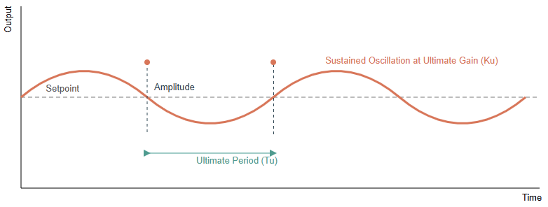
In the closed-loop Ziegler–Nichols method, integral and derivative gains are set to zero. The proportional gain is increased gradually.

This continues until the system reaches the ultimate gain. At this point, the system oscillates with constant amplitude. 

The oscillation period is recorded. This value is known as the ultimate period. Using these two values, PID gains are calculated.

Predefined formulas are used. This method is simple and fast. However, it often results in aggressive tuning. 

Significant overshoot is common. As a result, it is best suited for systems requiring fast response. Precision is less important in such cases.

Sustained oscillation waveform used to identify key parameters

Cohen–Coon Tuning Method

The Cohen–Coon method is another classical approach. It is particularly useful for processes with significant dead time.

This method relies on an open-loop step response. The response belongs to the system being controlled.

By applying a step input, the output is observed. Key parameters are then estimated. These include process gain, time constant, and dead time. These parameters are used in empirical formulas. The formulas calculate PID gains.

Compared to Ziegler–Nichols, Cohen–Coon often provides better performance. This is especially true for slow processes.

These processes usually have delays; however, it requires a reliable open-loop test. This may not always be feasible, and it may also be unsafe in industrial systems.

Frequency-Domain and Model-Based Tuning

For applications requiring higher precision, advanced tuning methods are used. These include frequency-domain and model-based approaches. These methods rely on mathematical models. The models represent the system.

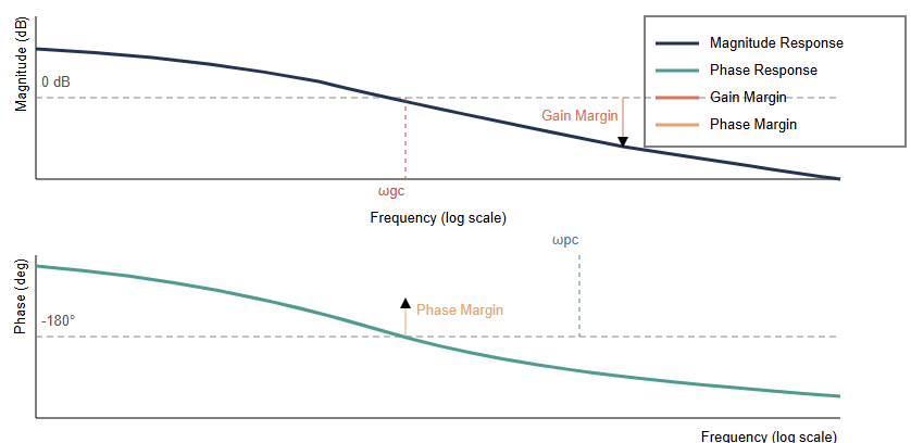
In frequency-domain tuning, tools such as Bode plots are used. Nyquist diagrams are also applied. These tools adjust PID gains.

The goal is to achieve desired gain and phase margins. This method provides strong insight into stability. 

It also improves robustness. However, it requires control theory knowledge. Accurate system modeling is also required. Model-based tuning involves identifying a mathematical model. 

The model represents the plant. PID parameters are computed using optimization techniques.

Many modern control software packages offer auto-tuning features. These features are based on these principles.

Bode plot illustrating gain margin and phase margin for PID tuning