PID stands for Proportional–Integral–Derivative, and remains the most widely used control algorithm in the global industry.

They are mainly used in industrial automation and robotics. Also, in areas such as power electronics and process control. 

Their popularity comes from a good balance between simplicity and robustness. Plus, the performance they offer.

They possess a very simple structure. However, correctly tuning PID controllers can be a big challenge. Poor tuning may result in excessive overshoot. 

It may cause slow response, oscillations, or even instability. On the other hand, a well-tuned PID controller can significantly improve system performance. It can reduce energy consumption and extend equipment life. 

Fundamentals of PID control are explained in the present article. It provides practical, step-by-step guidance on how to tune a PID controller. Both classical and modern methods are covered.

Understanding the PID Controller

A PID controller generates a control signal based on the error (E). The error is between the desired setpoint and the actual measured output.

The output belongs to a system. The error signal is processed through three distinct terms. 

These terms are proportional, integral, and derivative. Each term contributes differently to the controller’s behavior.

The proportional (P) term produces an output proportional to the current error. Increasing the proportional gain generally makes the system respond faster. Too much gain can cause oscillations or instability. 

The integral (I) term accumulates past errors over time. This term is responsible for eliminating steady-state error.

Excessive integral action can lead to slow response. It can also cause oscillatory behavior known as integral windup. 

The derivative (D) term predicts future error based on the rate of change. It improves damping and reduces overshoot. It is sensitive to noise and measurement disturbances.

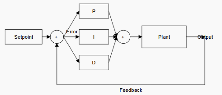
Block diagram of a PID controller

Objectives of PID Tuning

Before tuning a PID controller, it is important to understand good performance. Good performance depends on the specific application. Common performance objectives include rise time and settling time. 

They also include overshoot, steady-state error, and stability margin. Rise time refers to how quickly the system output reaches the desired setpoint.

Settling time measures how long the output takes to stabilize. Given a specific acceptable error band, this settling time must remain within it. 

Most of the time, the output may exceed the setpoint. This phenomenon is known as overshoot. This happens before the system stabilizes.

Steady state error describes the final difference between the output and the setpoint. Stability ensures that the system does not oscillate indefinitely.

It also ensures the system does not diverge. Different applications prioritize different objectives. For example, motion control systems often prioritize fast response.

They also aim for low overshoot. Temperature control systems may tolerate slower responses. However, they require high stability and minimal oscillation.

Preparing the System for Tuning

Proper system preparation is the foundation of successful PID tuning. The first step is to understand the nature of the process.

This process is the one being controlled. Determine whether the system is fast or slow. 

Also, check whether it is linear or nonlinear. Identify if it contains significant delays or dead time.

Verification of the proper calibration of sensors is a must. Make sure that noise is minimized. Actuators should operate within their limits. 

In addition, safety constraints must be clearly defined. It is also important to disable integral and derivative action initially.

This is recommended when starting most tuning procedures. This simplifies the process. 

It also reduces the risk of instability during early adjustments. If possible, perform tuning under normal operating conditions.

Tuning a controller at light load can cause problems. Unrealistic conditions can lead to poor performance. This poor performance appears during actual operation.

Manual PID Tuning Method

It is also called the Trial-and-Error method. Manual tuning is one of the most intuitive approaches.

It is also widely used in industrial environments. Although it may not produce mathematically optimal results, it is practical. It is effective for many systems.

The process usually starts by setting integral and derivative gains to zero. Increase the proportional gain gradually.

Continue until the system responds quickly. It should begin to oscillate slightly. At this point, reduce the proportional gain slightly. 

This helps achieve a stable response. The response should have an acceptable speed. Next, introduce integral action to eliminate steady-state error. Increase the integral gain slowly, and continue until the steady-state error is removed. 

This should occur within a reasonable time. Be cautious during this step. Too much integral gain can introduce oscillations. It can also cause sluggish behavior. Finally, add a derivative action to improve damping. 

It also helps reduce overshoot. Increase the derivative gain gradually. Continue until oscillations are minimized.

The transient response should become smoother. Excessive derivative gain should be avoided since it is sensitive to noise.

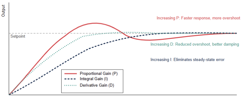
Step response plots showing the effect of increasing gains

Ziegler–Nichols Tuning Method

The Ziegler–Nichols method is one of the most well-known techniques. It is considered a classical tuning approach.

It provides systematic rules for selecting PID parameters. These rules are based on observed system behavior.

In the closed-loop Ziegler–Nichols method, integral and derivative gains are set to zero. The proportional gain is increased gradually.

This continues until the system reaches the ultimate gain. At this point, the system oscillates with constant amplitude. 

The oscillation period is recorded. This value is known as the ultimate period. Using these two values, PID gains are calculated.

Predefined formulas are used. This method is simple and fast. However, it often results in aggressive tuning. 

Significant overshoot is common. As a result, it is best suited for systems requiring fast response. Precision is less important in such cases.

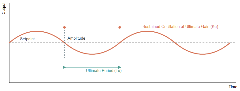
Sustained oscillation waveform used to identify key parameters

Cohen–Coon Tuning Method

The Cohen–Coon method is another classical approach. It is particularly useful for processes with significant dead time.

This method relies on an open-loop step response. The response belongs to the system being controlled.

By applying a step input, the output is observed. Key parameters are then estimated. These include process gain, time constant, and dead time. These parameters are used in empirical formulas. The formulas calculate PID gains.

Compared to Ziegler–Nichols, Cohen–Coon often provides better performance. This is especially true for slow processes.

These processes usually have delays; however, it requires a reliable open-loop test. This may not always be feasible, and it may also be unsafe in industrial systems.

Frequency-Domain and Model-Based Tuning

For applications requiring higher precision, advanced tuning methods are used. These include frequency-domain and model-based approaches. These methods rely on mathematical models. The models represent the system.

In frequency-domain tuning, tools such as Bode plots are used. Nyquist diagrams are also applied. These tools adjust PID gains.

The goal is to achieve desired gain and phase margins. This method provides strong insight into stability. 

It also improves robustness. However, it requires control theory knowledge. Accurate system modeling is also required. Model-based tuning involves identifying a mathematical model. 

The model represents the plant. PID parameters are computed using optimization techniques.

Many modern control software packages offer auto-tuning features. These features are based on these principles.

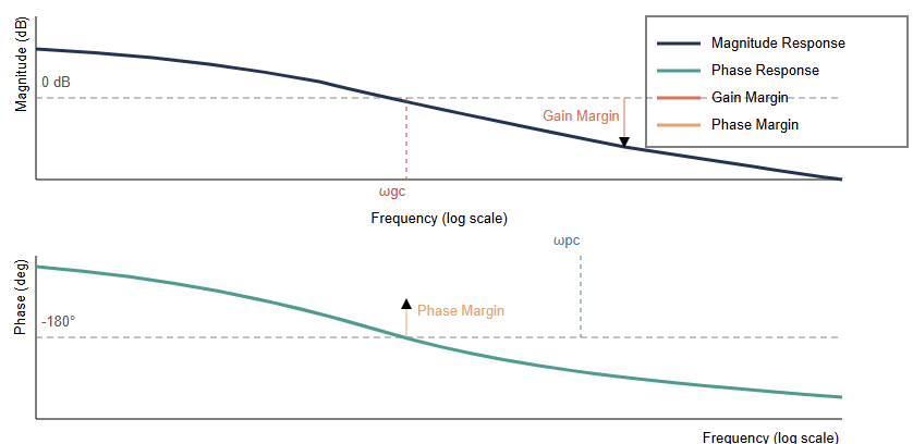
Bode plot illustrating gain margin and phase margin for PID tuning

Dealing with Integral Windup

Integral windup is a common problem in PID controllers. It is especially common when actuators saturate.

When the controller output is limited, problems arise. The integral term may continue to accumulate error. This leads to a large overshoot. 

The overshoot occurs once the system returns to normal operation. Anti-windup techniques are used to mitigate this issue. Common methods include clamping the integral term. 

Back-calculation is also used. Conditional integration is another method. Implementing anti-windup is essential for many systems.

This is especially true for systems with actuator limits. It is also important for frequent setpoint changes.

Effective PID Tuning: Practical Tips

Applying practical guidelines can improve tuning outcomes. Always make small changes to gain. Then observe the system response.

Document parameter changes and results, as it helps avoid confusion. Use filters on the derivative term. 

This reduces noise sensitivity. It is also important to consider sampling time. This applies to digital PID controllers. An inappropriate sampling period can degrade performance. 

It can also cause instability. Finally, remember that tuning is often iterative. Real-world systems may require periodic retuning. This is due to wear, load changes, or environmental variations.

Auto-Tuning and AI

Currently, many high-end PLCs feature Auto Tune buttons. PLCs are Programmable Logic Controllers that use relay oscillation techniques. The goal is to automatically determine optimal parameters.

Furthermore, AI-based tuning is emerging. These systems monitor the machine continuously.

They operate restlessly, and if a bearing starts to wear, adjustments are made. If a load changes, compensation is applied. 

The AI silently adjusts the PID values. This process compensates for system changes. This approach is known as adaptive control. The result is peak operational efficiency with reduced human intervention.

PID Tuning: Common Pitfalls to Avoid

Common issues during the tuning of a PID controller:

• Over-tuning: Trying to make a slow system behave like a fast one. A large oven should not act like a motor. This approach only leads to instability.
• Ignoring noise: Derivative action amplifies noise. If the sensor signal is not filtered, problems occur. The derivative gain can vibrate actuators excessively.
• Loop interaction: In complex factories, one PID loop may fight another. Always tune the innermost loop first. The most critical loop should be prioritized.

Conclusion

The present article covered the fundamentals of PID control. It provided practical guidance for tuning PID controllers.

Both classical and modern methods were discussed. Tuning a PID controller is both an art and a science. 

The underlying principles are well established. Real-world systems introduce uncertainties.

These uncertainties require practical judgment and experience. By understanding each PID term, engineers improve results. 

Clear performance objectives must be defined. Appropriate tuning methods should be applied.

This leads to stable and efficient control. Manual tuning has its place, in which a classical method like Ziegler–Nichols are useful. 

Modern model-based techniques are also valuable. With careful preparation and systematic adjustment, PID controllers deliver reliable control. They provide high-quality performance across many applications.

FAQ: How to Tune a PID Controller

What does “tuning a PID controller” mean?

Tuning a PID controller means choosing appropriate values for the proportional (P), integral (I), and derivative (D) gains so the controlled system responds well to changes in setpoint and disturbances, balancing speed, stability, and overshoot.

Why is PID tuning important?

Incorrect tuning can lead to oscillations, slow response, overshoot, or even instability. Proper tuning ensures predictable, efficient control and reduces wear on equipment.

What are the common methods for tuning a PID controller?

There are several methods, including manual trial-and-error, Ziegler–Nichols method, Cohen–Coon method, and software-based model tuning tools like MATLAB’s PID Tuner, which use response data to compute gains. 

What is the Ziegler–Nichols tuning method?

It’s a heuristic tuning approach where you set I and D to zero, increase P until sustained oscillation occurs, record the gain (Ku) and period (Tu), and then apply formulas to calculate P, I, and D gains. 

Should I start tuning with all gains at zero?

Yes. A common practical approach is to start with I and D at zero, increase P until the output responds and, if necessary, oscillates lightly, then bring in I to eliminate steady-state error and D to reduce overshoot.