controlcircuitry.com

All About Control Engineering

What Is The Difference between Ethernet IP and Modbus TCP

Posted on October 18, 2025 by Seki Hudson

In modern industrial automation, reliable communication between devices is essential.

Every process, from a simple sensor reading to a largescale production line, depends on seamless data exchange between controllers, sensors, and actuators.

Two of the most widely used Ethernet-based protocols are EtherNet/IP and Modbus TCP.

At first glance, they appear similar since both use standard Ethernet networks for communication.

However, beneath this shared foundation, they differ significantly in how they structure, transmit, and manage data.

This article details the key differences between EtherNet/IP and Modbus TCP, explaining their architectures, communication methods, performance, and best application areas.

It aims to help engineers, integrators, and system designers choose the right protocol for their specific needs based on speed, complexity, interoperability, and security.

Overview and Background

Ethernet-based communication has become the backbone of industrial control systems.

It provides high speed data exchange, easy scalability, and the ability to integrate multiple layers from field devices to enterprise networks on a single platform.

Both Modbus TCP and EtherNet/IP take advantage of these benefits but in different ways.

Modbus TCP is valued for its simplicity and openness. It builds upon the traditional Modbus protocol and adapts it to modern Ethernet networks.

WhileEtherNet/IP, on the other hand, is feature-rich and powerful. It brings advanced capabilities from the Common Industrial Protocol (CIP), enabling real-time control, motion coordination, and system wide integration.

Understanding how each protocol works is essential to designing reliable automation systems that balance cost, performance, and scalability.

Architecture and Data Model

In this section we will review an architecture and data model of each of these communication protocols.

Modbus TCP

Modbus TCP is one of the easiest industrial communication protocols to implement.
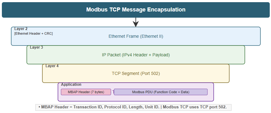
It is an open standard that encapsulates the traditional Modbus RTU frame inside a TCP/IP packet.

So, this allows it to function over Ethernet without major modifications.

Key features:

Based on a client-server (or master-slave) communication model.
The client initiates a request; the server processes it and sends a response.
Data is represented in simple tables known as registers and coils.

Common data types:

Coils: Discrete on/off values used for digital outputs.
Input Status: Read only discrete inputs.
Holding Registers: 16-bit read/write registers used for analog values or process data.
Input Registers: 16-bit read-only registers used for sensor input data.

Each device on a Modbus TCP network is identified by a unique IP address. For systems connected through gateways to Modbus RTU networks, a Unit Identifier is used to route messages to the correct device.

A Modbus TCP message includes:

A 7-byte MBAPheader (Modbus Application Protocol header).
The Protocol Data Unit (PDU), which contains the function code and data.
The entire message is encapsulated inside a TCP/IP frame and transmitted via Ethernet.

This simple and consistent structure makes Modbus TCP highly transparent, easy to debug, and compatible with many devices and software tools.

EtherNet/IP

EtherNet/IP (Ethernet Industrial Protocol) is more sophisticated. It adapts the Common Industrial Protocol (CIP) to Ethernet, providing a consistent way to model data, manage devices, and control real-time operations.

Unlike Modbus TCP’s table based design, EtherNet/IP is object-oriented. Devices organize their data into logical objects, each containing multiple attributes that represent different parameters or values.

Communication models:

ExplicitMessaging (Client/Server): Used for configuration, diagnostics, and non-time-critical data. Operates over TCP for reliable delivery.
ImplicitMessaging (Producer/Consumer): Used for real-time I/O data exchange. Operates over UDP for high-speed, cyclic, multicast communication.

Addressing:

Devices are identified by IP addresses.
Specific data is accessed through a CIP path, which points to the object and attribute to be read or written.

Port usage:

TCP port 44818 for explicit messaging.
UDP port 2222 for implicit messaging.

Because of its object-oriented structure, EtherNet/IP supports complex applications such as synchronized motion control, advanced diagnostics, and flexible system integration.

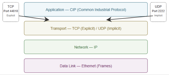
Key Differences Between EtherNet/IP and Modbus TCP

While both protocols share Ethernet as a physical medium, their operation and capabilities differ considerably.

Main distinctions

Data Model

EtherNet/IP: Object-oriented using CIP; Modbus TCP: Simple, table based registers and coils.

Communication Style

EtherNet/IP: Producer/Consumer (implicit) and Client/Server (explicit); Modbus TCP: Client/Server only.

Real-Time Performance

EtherNet/IP: Excellent real-time behavior using UDP implicit messaging; Modbus TCP: Limited real-time capability; sequential requests can slow communication.

Addressing

EtherNet/IP: IP address plus CIP path; Modbus TCP: IP address plus Unit Identifier.

Openness

EtherNet/IP: Managed by ODVA, which may require vendor certification; Modbus TCP: Completely open and royalty-free.

Complexity

EtherNet/IP: More complex configuration and setup; Modbus TCP: Very easy to implement.

Security

EtherNet/IP: Supports CIP Security (authentication, encryption, and access control); Modbus TCP: Lacks built-in security, depends on network firewalls or VPNs.

Troubleshooting

EtherNet/IP: Requires specialized diagnostic tools; Modbus TCP: Easier to analyze and debug with standard tools.

Flexibility and Use Case

EtherNet/IP: Best for complex, large-scale systems and motion control; Modbus TCP: Ideal for simple monitoring and legacy equipment.

Performance and Reliability

Speed and Determinism

Real-time performance is one of the main criteria for choosing between these protocols.

Modbus TCP

Relies on TCP, which guarantees reliable delivery but can introduce variable delays.

Each client must wait for a response before sending a new request, which increases scan time as more devices are added.

Suitable for non-time-critical monitoring but not for synchronized control.

EtherNet/IP

Achieves faster and more deterministic performance through implicit messaging.

UDP allows multicast communication, enabling one device to send updates to many consumers simultaneously.

This model reduces network load and increases efficiency for real-time control.

Traffic can also be prioritized using Quality of Service (QoS) to maintain predictable timing.

Reliability and Error Handling

Both rely on Ethernet and TCP/IP layers for basic reliability.
However, EtherNet/IP adds extra diagnostic and error-handling capabilities.

Modbus TCP:

Simplicity means fewer error management features.
TCP ensures packet delivery, but application-level fault handling is minimal.

EtherNet/IP:

Includes mechanisms for connection supervision, timeouts, and controlled disconnections.
Explicit messages can terminate safely if errors occur.
Implicit connections can detect timeouts and re-establish communication automatically.

Security Considerations

As industrial systems become more connected, cybersecurity is critical.

Modbus TCP:

Designed in the 1990s when network threats were minimal.
Does not include built-in authentication, authorization, or encryption.
Vulnerable to attacks if exposed to public networks.
Recommended protection includes network segmentation, VPNs, and firewalls.

EtherNet/IP:

Incorporates CIP Security, which aligns with modern industrial cybersecurity standards.
Features include:
- Authentication: Verifies the identity of communicating devices.
- Encryption: Secures the data transmitted between devices.
- Access Control: Restricts communication to approved connections.
These features make EtherNet/IP suitable for applications where security and data integrity are mandatory.

Implementation and Configuration

Modbus TCP

One of Modbus TCP’s greatest strengths is its simplicity.
It can be configured within hours by engineers familiar with TCP/IP networks.

Typical setup steps include: Assigning IP addresses to devices, mapping registers for reading and writing data and finally, defining the function codes required by the client.

Because of its simplicity, Modbus TCP is ideal for small or medium-sized projects, quick prototyping, and systems where minimal configuration time is preferred.

EtherNet/IP

EtherNet/IP offers much greater flexibility but requires more effort to configure.
It involves defining objects, services, and I/O connections within the CIP framework.

Specialized tools from vendors such as Rockwell Automation are often used to configure and diagnose networks.

While the initial setup takes longer, the reward is advanced performance, scalability, and tight integration between devices.

Hardware and Interoperability

Both protocols use standard Ethernet hardware such as switches, routers, and network interface cards.
However, their interoperability and hardware requirements differ slightly.

Modbus TCP:

Uses standard, low-cost Ethernet components.
Widely supported across vendors and compatible with older Modbus RTU devices via gateways.
Excellent for mixed environments that include legacy systems.

EtherNet/IP:

Also based on Ethernet, but devices may require more processing power to handle CIP messaging and real-time tasks.
Certified by ODVA, ensuring consistency and interoperability between manufacturers.
Preferred in systems built around Rockwell Automation or similar high-end control environments.

Choosing the Right Protocol

The decision between EtherNet/IP and Modbus TCP depends on project needs, device compatibility, and performance expectations.

Choose Modbus TCP when:

You are integrating legacy or simple devices.
The system involves basic data acquisition or monitoring.
Cost and ease of implementation are top priorities.
Real-time performance is not critical.
You need a protocol that works across many vendors with minimal setup.

Choose EtherNet/IP when:

The application demands high-speed or synchronized control.
The network involves robotics, motion systems, or large-scale automation.
You need strong security and diagnostic features.
You require seamless integration across multiple system levels using CIP.
Long-term scalability and performance are essential.

Key Takeaways: The Difference between Ethernet IP and Modbus TCP

This article detailed how both EtherNet/IP and Modbus TCP play vital roles in modern industrial communication.

They share Ethernet as a common platform but serve different purposes depending on system complexity and performance needs.

Modbus TCP stands out for its simplicity, openness, and low cost. It is well suited for basic monitoring, energy management, and legacy system integration.

Its straightforward structure makes it easy to implement, maintain, and troubleshoot with minimal technical effort.

EtherNet/IP excels in speed, flexibility, and security. Its object-oriented model, support for real-time communication, and advanced protection features make it ideal for high-end automation, motion control, and large distributed systems.

Choosing between the two depends on balancing performance, complexity, security, and budget.

For small or cost-sensitive projects, Modbus TCP offers a reliable and simple solution.

On the other hand, for large, performance critical environments, EtherNet/IP provides the power, scalability, and precision required by modern industries.

FAQ: The Difference between Ethernet IP and Modbus TCP

What is EtherNet/IP?

EtherNet/IP adapts the Common Industrial Protocol (CIP) to Ethernet, supporting object-oriented data and real-time control.

What is Modbus TCP?

Modbus TCP wraps the Modbus protocol in a TCP/IP packet, enabling Modbus messaging over Ethernet.

Which protocol supports real-time control better?

EtherNet/IP, via its UDP-based implicit messaging, provides more deterministic performance.

Which is simpler to implement?

Modbus TCP is simpler, with fewer layers and a straightforward request/response model.

What about security?

EtherNet/IP supports CIP Security (authentication, encryption), while Modbus TCP lacks built-in security.

How do they address data?

EtherNet/IP uses IP + CIP path to reach objects/attributes. Modbus TCP uses IP + Unit Identifier to map to registers.

Are both open standards?

Modbus TCP is fully open and royalty-free. EtherNet/IP is governed by ODVA and may require compliance or certification.

When should I choose Modbus TCP?

Use Modbus TCP for simple data acquisition, legacy device support, or when cost and ease matter more than performance.

When is EtherNet/IP preferred?

Choose EtherNet/IP for high-speed control, synchronized operations, and complex automation with security needs.

How a Pressure Transmitter Works with PLCs

Posted on October 18, 2025 by Seki Hudson

In modern industrial automation, precise monitoring and control depend on the smooth communication between field devices and controllers.

One of the most important examples is the integration of a pressure transmitter with a Programmable Logic Controller (PLC).

A pressure transmitter converts a physical pressure value into a standard electrical signal, usually 4–20 mA, that the PLC can interpret.

The PLC then uses this signal to make decisions, such as opening a valve, activating a pump, or triggering an alarm.

This interaction forms the foundation of automated systems in industries like manufacturing, chemical processing, oil and gas, and water treatment. The result is better efficiency, improved safety, and greater reliability.

This article details how a pressure transmitter works with a PLC, explaining the signal conversion process and integration steps.

It also introduces best practices, and common troubleshooting methods used in industrial automation.

Pressure Signal to PLC Program

The path from a process’s actual pressure to PLC decision making involves three main stages: Pressure sensing at the source, signal conversion and transmission and PLC processing and control

In the following subsections we will take a look at each step, in detail.

Pressure Sensing at the Source

The first task of a pressure transmitter is to sense the actual pressure of a fluid either gas or liquid.

Inside the transmitter, a sensing element (often a diaphragm) deflects slightly in response to changes in pressure.

This mechanical deflection is the basis for the measurement. Different transmitters measure different pressure types:

Gauge Pressure: Compares pressure to the surrounding atmosphere.
Absolute Pressure: Compares pressure to a perfect vacuum.
Differential Pressure: Measures the difference between two separate pressure points, such as across a filter or tank.

Converting Pressure to Electrical Signal

Once the pressure is sensed, the transmitter’s internal electronics convert it into a standardized electrical signal.

The most widely used output is the 4–20 mA current loop. It’s preferred because current signals resist electrical noise and remain stable over long cable distances.

How the 4–20 mA Loop Works:

The transmitter typically operates as a 2-wire device.
The same two wires provide both power and signal.
The PLC supplies 24 V DC to power the transmitter.
The transmitter modulates the current between 4 mA (minimum) and 20 mA (maximum) to represent the measured pressure.
- 4 mA = 0% of the pressure range
- 20 mA = 100% of the pressure range
- 12 mA = approximately 50% of the range
This current signal travels to the PLC’s analog input module, which measures it.

PLC Processing and Control

The PLC’s analog input module converts the received 4–20 mA signal into a digital integer value.

This raw number must be scaled into real world engineering units like bar or psi so that the control logic can use it.

Scaling the Input

Scaling converts the raw input into readable engineering values. The general formula is:

For example: 4 mA = 0 bar; 20 mA = 10 bar; A midrange signal (12 mA) represents about 5 bar.

Once scaled, the PLC program uses this value for decision making.

Executing Control Logic

The PLC compares the scaled pressure with pre-set limits:

If the pressure drops below a lower limit, it may start a pump.
If it rises above a high limit, it can shut down equipment or trigger alarms.

This ensures safe, automatic operation and reduces the need for manual intervention.

Integrating the Pressure Transmitter with a PLC

Integration requires correct hardware selection, proper wiring, and accurate software configuration.

Step 1 – Selecting the Right Hardware

Choose a pressure transmitter that fits the process requirements:

Pressure Type: Gauge, absolute, or differential
Range: The expected operating pressure range
Accuracy: Depending on process criticality
Material Compatibility: Must match the process fluid

Also, ensure that the PLC’s analog input module supports the same signal type (e.g., 4–20 mA). Some modules accept voltage signals, so compatibility is important.

Step 2 – Wiring the Components

Before wiring, turn off all power sources and follow lockout/tagout safety procedures.

Connecting a 2-Wire Transmitter:

Connect the positive (+) terminal of the 24 V DC power supply to the positive (+) terminal of the transmitter.
Connect the negative (–) terminal of the transmitter to the analog input channel of the PLC.
Connect the common terminal of the analog input module back to the negative (–) terminal of the power supply.

This completes the current loop.

Grounding: Proper grounding is essential. It prevents electrical noise and ensures accurate signal transmission.

Step 3 – Configuring the PLC

Set the Input Range:

In the PLC’s hardware configuration, define the analog input channel as 4–20 mA. This ensures the PLC interprets the signal correctly.

Apply Scaling:

Use scaling blocks or math functions in the PLC program to convert the raw digital input into engineering units.

This allows operators to see the actual pressure on the HMI (Human-Machine Interface).

Define Alarms and Logic:

Program the PLC to take specific actions when pressure limits are reached:

Low-pressure alarm: Warns or starts a pump
High-pressure alarm: Shuts off valves or stops pumps
Critical limit: Activates an emergency shutdown (ESD)

These logic steps transform raw data into actionable control.

Best Practices and Troubleshooting

Even well-designed systems can experience issues. Following installation best practices helps prevent problems and improves accuracy.

Best Practices

Avoid Electrical Noise

Use shielded cables and route them away from power cables or variable frequency drives (VFDs).

Stable Mounting

Install transmitters away from vibration, heat, or direct sunlight.

Regular Calibration

Calibrate transmitters periodically to maintain accuracy. Calibration involves applying known pressures and adjusting the transmitter’s zero and span.

zero and span.

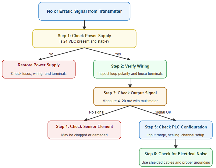
Common Problems and Solutions

Problem	Possible Cause	Solution
No signal (4 mA constant)	No power, broken wire, or blocked sensor	Check power supply, wiring, and sensor diaphragm
Full signal (20 mA constant)	Pressure exceeds range or calibration error	Verify process pressure and recalibrate
Erratic reading	Electrical noise, loose wiring, or vibration	Check shielding, grounding, and mounting

Advantages of PLC-Integrated Pressure Transmitters

Connecting pressure transmitters to PLCs brings multiple operational benefits.

Enhanced Process Control

Real-time data allows for precise and automated adjustments. Processes stay consistent and efficient, ensuring stable production quality.

Increased Safety

Continuous monitoring detects unsafe pressure levels early. PLCs can immediately shut down equipment or trigger alarms to prevent damage or accidents.

Better Data and Analytics

PLCs can log and trend pressure data. Engineers use this information to optimize performance, predict maintenance needs, and detect gradual system degradation.

Reduced Costs

Optimized operations lower energy consumption, reduce waste, and minimize downtime. Over time, these savings justify the investment in automation.

Case Study: Tank Level Monitoring Using a Differential Pressure Transmitter

To understand this integration in practice, consider a chemical plant where a PLC maintains the level in a storage tank using a differential pressure (DP) transmitter.

Measurement

The DP transmitter measures the pressure difference between the bottom and the top of the tank.

This difference corresponds directly to the liquid height, since pressure at the base depends on fluid density and height.

Signal Transmission

The transmitter converts this pressure difference into a 4–20 mA signal and sends it to the PLC’s analog input.

PLC Logic

The PLC reads the 4–20 mA signal.
It scales it into engineering units (for example, 0–10 meters of tank level).
The ladder logic then executes the following:
- If the tank level falls below 20%, the PLC turns on a pump to refill.
- When the level reaches 90%, the pump turns off.
- If the level exceeds 95%, a high-level alarm activates.

Control Outcome

This automation keeps the tank level within a safe and efficient range.
It prevents overflow, reduces waste, and ensures continuous production without manual intervention.

Key Takeaways: How a Pressure Transmitter Works with PLCs

This article introduced how a pressure transmitter works with a PLC, by detailing the signal conversion process and integration steps.

In addition, it studied the best practices, and common troubleshooting methods used in industrial automation.

This leads to conclude that the pressure transmitter–PLC system is a cornerstone of industrial automation.

It transforms physical pressure into a digital signal that drives intelligent control decisions.

By following correct installation steps, configuring inputs properly, and maintaining calibration, engineers can create accurate, efficient, and safe control systems.

The ability of PLCs to interpret and act on pressure data enables smarter factories, where processes are optimized, downtime is minimized, and safety is always prioritized.

From simple tank monitoring to complex process control, the integration of pressure transmitters and PLCs continues to power the future of industrial automation.

FAQ: How a Pressure Transmitter Works with PLCs

What is the difference between a pressure transducer and a pressure transmitter?

A pressure transducer converts pressure into a small electrical signal (e.g., voltage or resistance).
A pressure transmitter includes signal conditioning and outputs a standardized signal (often 4–20 mA) that is easier for PLCs or other control systems to read.

Why is the 4–20 mA current loop standard used for transmitters?

The 4–20 mA loop is resistant to electrical noise over long cable distances, making it reliable in industrial environments.
The current loop can both power the transmitter and carry the signal (in two-wire devices).
Because the signal is current (not voltage), voltage drops in the wires don’t alter the reading.

How is a pressure transmitter wired to a PLC?

Most transmitters use two-wire wiring: the same pair carries power (often 24 V DC) and the signal (4–20 mA) to the PLC’s analog input.
Some transmitters are four-wire types: separate wires for power and signal.
In wiring, you must configure the PLC analog input module for current input and connect the loop correctly (positive end to transmitter, negative back to PLC).
Modules often support single-ended or differential wiring modes, affecting how you route the wires.

How is the transmitter signal converted into meaningful pressure values in the PLC?

The PLC’s analog input module reads the 4–20 mA current and converts it to a raw digital count (integer).
Then you apply a scaling formula in the PLC logic to map raw counts to engineering units (e.g., psi, bar).
For example, if your card is 14-bit (0 to 16,383 counts), the formula would subtract the counts representing 4 mA, divide by the span (counts for 4–20 mA), then multiply by the max pressure.

What pressure types can the transmitter measure?

Gauge pressure (relative to ambient atmospheric pressure)
Absolute pressure (relative to vacuum)
Differential pressure (difference between two pressure points)

Selecting the right type depends on your application (tank level, flow, sealing, etc.).

What are common errors or issues when integrating transmitters with PLCs?

No output (4 mA stuck): Could be broken wiring, incorrect power supply, or a failed transmitter.
Max output (20 mA stuck): Could mean pressure outside range, calibration error, or internal fault.
Unstable or noisy readings: Often due to electrical noise, improper grounding, or poor shielding of wiring.
Incorrect scaling / mapping: If scaling is set wrong, the displayed pressure is incorrect. Check the formula and calibration points.

How often should the pressure transmitter be calibrated?

Routine calibration is recommended to maintain accuracy over time, especially in critical processes.
Calibration involves applying known pressures, checking zero and span, and adjusting as needed.

Can the transmitter be cleaned or repaired?

Cleaning: Yes, but with care. Use a soft cloth with alcohol or lukewarm water. Do not submerge or damage the sensor face.
Repair: Possible, but typically handled by specialists or manufacturers. Internal parts (strain gauges, electronics) are delicate.

What is a span vs. range in transmitter terms?

The range is the lowest to highest pressure the device is specified to measure (e.g., 0–100 psi).
The span is the difference between the highest and lowest values (so range = 0 to 100 psi gives a span of 100 psi).

Can a PLC read multiple transmitters from a single power supply?

Yes. In many cases, multiple two-wire transmitters can share a single 24 V DC supply, each looped to a separate analog input channel, as long as the power supply’s capacity is sufficient.

PLC Counters Explained with Examples

Posted on October 18, 2025 by Seki Hudson

In industrial automation, Programmable Logic Controllers (PLCs) are vital for managing machines and processes. Among their key functions is counting tracking events, pulses, or signals from inputs.

PLC counters act as digital versions of mechanical tally counters, offering reliable, flexible, and maintenance free control. Unlike mechanical counters, PLC counters operate in software.

This allows precise and programmable logic adaptable to many tasks, such as packaging, material handling, and inventory control.

This article explains what PLC counters are, their types, components, and practical ladder logic examples.

It also highlights advanced features and best practices for ensuring accuracy and efficiency in automated industrial systems.

What is a PLC Counter?

A PLC counter is an internal software instruction used to keep track of the number of times a specific event occurs during a process.

Rather than relying on a physical mechanism with gears or springs, it uses the PLC’s memory to store numerical data that changes according to input signals.

Each time an assigned input changes state from a logic “0” to a logic “1”, the counter either increments or decrements its accumulated value (AV).

When this value reaches a predetermined limit known as the preset value (PV), the counter’s done bit activates.

This “done” condition can then be used to trigger another event in the program. This event could be such as stopping a motor, activating an alarm, or initiating another machine cycle.

By performing counting functions in software, PLC counters ensure precision and repeatability.

They are easy to configure for different operations such as batch production, product tracking, or sequential control.

They are also highly reliable because they have no moving parts. This means they are not affected by wear or vibration, problems that often occurred with older mechanical counters.

In short, a PLC counter serves as a digital event tracker, allowing a system to respond automatically once a specific number of occurrences is detected.

Types of PLC Counters

PLCs typically include three main types of counters, each suited to a particular kind of counting behavior:

Count-Up (CTU) Counter

Function: The CTU counter increases its stored or accumulated value by one every time the assigned input transitions from false to true.
Operation: As pulses are received, the counter continues to increment until its accumulated value equals or exceeds the preset number set by the programmer. Once this happens, the counter’s done bit (DN) is activated and can trigger another output or sequence.
Reset: The counter can be reset at any moment using its reset input, which clears the accumulated value back to zero.
Application Example: Suppose a conveyor belt system needs to count 10 items before activating a packaging robot. Each time a sensor detects an item, the CTU counter increases by one. Once the total reaches ten, the done bit becomes true, signaling the robot to pick up the batch and start the packaging cycle.

Count-Down (CTD) Counter

Function: The CTD counter performs the opposite task—it decreases its accumulated value by one each time an input pulse is detected.
Operation: This type of counter is usually initialized with a preset value and counts down toward zero. When the accumulated value reaches zero, the counter’s done bit is set to true, signaling completion.
Load/Preset: Instead of a basic reset, CTDs often include a load (LD) input that reloads the preset value into the counter at the start of each new cycle.
Application Example: Imagine a dispenser containing 50 parts. The counter starts at 50 and decreases each time an item is released. When it reaches zero, the done bit activates a warning light or alarm to indicate the container is empty and needs refilling.

Count-Up/Count-Down (CTUD) Counter

Function: A CTUD counter combines the functions of both CTU and CTD. It can increase or decrease the same accumulated value depending on which input (up or down) receives a pulse.
Operation: The counter adds one count whenever the “up” input is activated and subtracts one count when the “down” input is triggered. Both inputs share the same memory location, which makes it ideal for processes that require two-way counting.
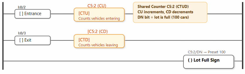
Application Example: Consider a parking garage that can hold 100 vehicles. A sensor at the entrance adds one count when a car enters, while a sensor at the exit subtracts one when a car leaves. The current value of the counter shows how many spaces are occupied. When the count reaches 100, the done bit triggers the “Lot Full” indicator.

Main Components of a PLC Counter

Although their specific implementation may differ among PLC brands, all counters have a common structure consisting of several key parts:

Counter Address or Tag: The unique identifier for the counter within the PLC program (e.g., C5:0 in Allen-Bradley PLCs).
Preset Value (PV): The target or limit that determines when the counter’s done bit should activate.
Accumulated Value (AV): The running count that changes as the input pulses occur. For CTU counters, it starts at zero; for CTD counters, it usually begins at the PV.
Done Bit (DN): A status flag that becomes true when the AV meets the preset condition.
Count-Up (CU) and Count-Down (CD) Inputs: The terminals or logical inputs that receive external pulses from sensors or switches.
Reset (R) or Load (LD): Inputs used to clear or reload the counter’s AV.

These elements make it easy for engineers to configure, monitor, and debug counting functions directly within the PLC software interface.

PLC Counter Examples Using Ladder Logic

Ladder Logic is the most widely used PLC programming language. This is because its visual structure resembles traditional electrical circuits, making it intuitive for technicians and engineers.

The following examples demonstrate how counters are typically implemented.

Example 1: Simple Count-Up Application (Part Counting)

Scenario: A machine must fill a box with 10 parts before sealing it. Each time a part is detected by a proximity sensor, the PLC increments a counter.
Logic: A CTU counter is programmed with a PV of 10. When the AV reaches this value, the DN activates the sealing mechanism.

Explanation:
The sensor sends a pulse every time a part enters the box, increasing the counter by one. Once the counter reaches 10, the DN energizes the output coil controlling the box-seal motor.

Example 2: Count-Down Application (Dispenser Control)

Scenario: A dispenser holds 25 items, and each item dispensed should reduce the count. When the counter reaches zero, a refill indicator turns on.
Logic: A CTD counter with a preset of 0 and an initial accumulated value of 25 is used.

Explanation:
Every time an item is dispensed, the sensor sends a pulse that decreases the accumulated value by one. When the counter reaches zero, the DN energizes the refill light, prompting an operator to restock the dispenser.

Example 3: Count-Up/Down Application (Parking Garage)

Scenario: A garage accommodates 100 cars. The system must track entries and exits to display a “Lot Full” signal when the capacity is reached.
Logic: A CTUD counter is used, with one sensor connected to the count-up input (entrance) and another to the countdown input (exit).

Explanation:
Each incoming car triggers the count up input; each departing car triggers the countdown input.

When the counter equals the PV of 100, the DN activates the “Lot Full” sign. When cars exit, the counter decreases accordingly, automatically turning the sign off.

Advanced Counter Concepts

Cascading Counters

When a single counter cannot handle very large numbers due to memory limits, multiple counters can be connected or cascaded.

The done bit of one counter acts as the input pulse for the next, effectively multiplying their counting capacity.

For example, cascading two counters each preset to 100 can extend the range up to 10,000 counts (100 × 100).

This approach is useful in applications such as production line totals or large-scale event monitoring.

High-Speed Counters (HSCs)

Standard PLC counters operate based on the PLC’s scan cycle. If input pulses occur faster than the scan rate, some may be missed.

To handle high-frequency signals, many PLCs offer High-Speed Counter (HSC) modules.

These modules process inputs directly through dedicated hardware, bypassing the main CPU to ensure no pulses are lost.

HSCs are essential for applications where precision timing and fast response are critical.

Examples of these applications are encoder feedback, speed measurement and/or motion control.

Best Practices for Using PLC Counters

Simulate Before Deployment

Test all counter logic in a simulation environment before implementing it in a real system to detect logic or wiring mistakes early.

Manage Reset Logic Carefully

Ensure that counters only reset when appropriate conditions are met, such as when a new production batch begins.

Use Descriptive Names

Assign meaningful tags such as Bottle_Count or Parts_Total to make the program easier to understand and maintain.

Prevent Overflows and Underflows

Always verify that the counter’s accumulated value stays within its valid range to avoid errors.

Use Suitable Hardware

When dealing with fast pulses or encoder signals, use high-speed counter modules to maintain accuracy.

Document Your Program

Include comments that describe each counter’s purpose and preset values to assist future troubleshooting or system updates.

Key Takeaways: PLC Counters

This article explained what PLC counters are and described their types and components.

It also presented real-life ladder logic examples. PLC counters are essential and versatile tools in modern industrial automation.

They form the foundation for many control tasks, from simple part counting on assembly lines to complex batch control operations.

By learning how to use CTU, CTD, and CTUD counters, engineers can design reliable and efficient automation systems.

Understanding their internal components and applying them correctly in ladder logic ensures error-free performance.

Modern PLCs now include High-Speed Counters and advanced communication features.

These improvements expand the use of precise counting in industrial systems. As automation grows more data-driven, accurate counting becomes increasingly important.

In today’s factories, the PLC counter remains a key element, ensuring every pulse, product, and process is tracked with precision.

FAQ: PLC Counters Explained

What is a PLC counter, and what are its basic parts?

A PLC counter is a software instruction that tracks pulses or events.
Main parts:
– CU/CD inputs: count up or down.
– PV: preset value or target count.
– CV/AV: accumulated value.
– Reset/Load: clear or set a starting value.
– Done bit: activates when preset is reached.

What types of PLC counters are there?

– CTU: counts up (e.g., parts on a conveyor).
– CTD: counts down (e.g., items remaining).
– CTUD: counts up and down (e.g., parking lot cars).

What are limits and overflow/underflow?

Each counter has max/min limits. Too many pulses can cause overflow or missed counts.

How does reset or load work?

Reset clears the count; Load sets an initial value.

What’s the difference between “normal” vs “high-speed” counters?

Normal counters rely on scan time; high-speed ones handle fast pulses independently.

How do counters behave on first scan or power-up?

Counters usually start at 0 (CTU) or PV (CTD). Some retain memory after power loss.

How do I ensure counting is accurate (i.e., avoid false/multiple counts)?

Use edge detection, debounce sensors, and ensure reset conditions are correct.

What happens when the preset value is changed during operation?

Altering PV during operation may instantly activate the done bit or need reset.

Can counters count negative values?

Some PLCs allow negative counts; others stop at zero.

Are there practical examples or applications of counters in industry?

Used for part counting, inventory tracking, maintenance cycles, and quality control.

What are status bits like overflow, underflow, done, etc.?

– DN: done.
– Overflow/Underflow: count exceeds limits.
– CU/CD: indicate direction of counting.

What features differ across brands / manufacturers?

Vary by count range, memory retention, speed, and handling of reset/load or high-speed features.

Learn how to program PLC here

PLCs vs DCS vs SCADA: Key Differences, Advantages, and Applications Explained

Posted on October 18, 2025 by Seki Hudson

Industrial automation relies on various control systems that help industries manage complex processes, equipment, and machinery efficiently. Among the most widely used are Programmable Logic Controllers (PLCs), Distributed Control Systems (DCS), and Supervisory Control and Data Acquisition (SCADA) systems.

These technologies share the common goal of enhancing productivity, reliability, and safety within industrial operations. However, they differ in terms of design, functionality, and application scale.

Understanding these distinctions is essential for selecting the right system for a specific process.

This article explores the main characteristics of each system, their advantages, and how they integrate to form a unified automation strategy in modern industrial environments.

What is a PLC?

A Programmable Logic Controller (PLC) is a digital industrial computer used for specific control tasks.

It is designed for reliability and to replace old relay-based systems. A PLC uses memory to store instructions that perform logic, timing, and sequencing functions.

PLC architecture

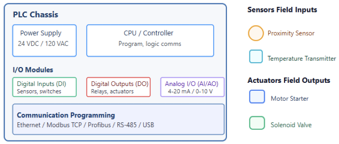
A typical PLC has a modular design. It includes a power supply, a CPU (Central Processing Unit), and input/output (I/O) modules (See Figure).

CPU

The CPU is the main processor. It interprets input signals and runs the control program.

I/O modules

These connect the PLC to the field. Inputs read sensors or switches, while outputs control actuators, motors, or valves.

Programming software

PLCs are programmed with specialized software using languages like ladder logic, function block diagrams or structured text.

Key characteristics of PLCs

Discrete control: Best for on/off and repetitive actions, like assembly lines or packaging systems.
High speed: Provides quick and predictable control cycles.
Local control: Usually manages one machine or process at a time.
Cost-effective: Ideal for small-scale control applications.

Advantages and disadvantages of PLCs

Advantages

Fast and deterministic control for critical tasks.