A PID controller is the brain behind many automated processes. It helps a system automatically maintain a specific target, or “setpoint,” with great accuracy.

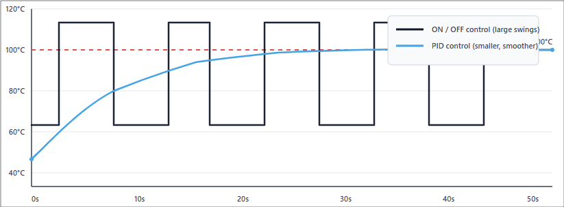
Unlike a simple ON/OFF switch, which can cause large swings, a PID uses a clever formula to make smooth, precise adjustments.

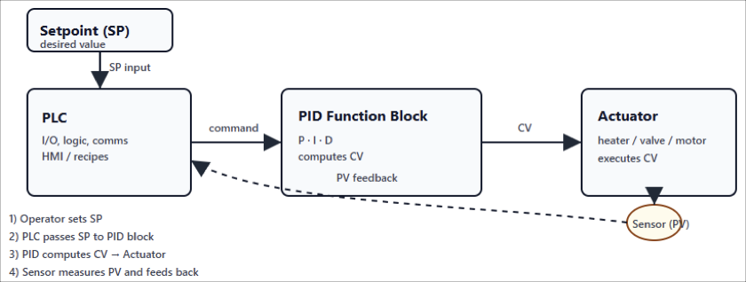
 In industrial settings, PID control is often run by a Programmable Logic Controller (PLC).

The PLC executes the PID algorithm and translates its calculations into commands that control machinery. 

This article will explain the core concepts of PLC PID control. It will break down how the “Proportional,” “Integral,” and “Derivative” terms work together to create a feedback loop that achieves and maintains a setpoint. 

We will explore the common challenge of “tuning” and provide practical examples of how PLC PID control is used in the real world. 

The Problem with Simple Control

Let’s begin with a relatable example: controlling the temperature in an oven. In the simplest system, this works like a light switch:

• The oven’s setpoint is the desired temperature.
• A sensor measures the current, actual temperature.
• If the temperature is too low, the controller turns the heater ON.
• If the temperature is too high, the controller turns the heater OFF.

This strategy is known as ON/OFF control. It is simple, but it has a big problem. It causes constant swings above and below the setpoint. The heater overshoots, then shuts off, then undershoots, and the cycle repeats.

This leads to inefficiency. The equipment experiences more stress and wears out faster.

For processes where high precision matters, like chemical reactions or semiconductor manufacturing, this is unacceptable.

That is why industries use PID control. It takes a smarter approach, one that reduces oscillations and provides smoother, more accurate control.

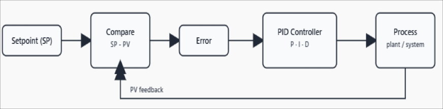
The Foundation: The Feedback Loop

At the heart of PID control lies a feedback loop. This is the continuous cycle where the system checks itself, compares values, and makes corrections.

There are four key parts to understand:

Setpoint (SP)

The target value. For example, keeping an oven at exactly 100 °C.

Process Variable (PV)

The actual measured value. This comes from a sensor, like a thermometer.

Error (E)

The difference between the setpoint and the process variable. Formula: E = SP – PV.

Control Variable (CV)

The output signal calculated by the PID algorithm and sent by the PLC to the equipment. For an oven, this could be the amount of power delivered to the heater.

The goal of the PID controller is simple in theory: make the error as close to zero as possible.

But in practice, achieving that balance requires the three components: P, I, and D — to work together. Each has a unique role in shaping how the system reacts.

The P, I, and D Explained

Proportional Term (P) – Reacting to the Present

The Proportional term is the most direct part of the equation. It creates a correction that is proportional to the size of the error.

• If the error is big, the correction is big.
• If the error is small, the correction is small.
• As you approach the setpoint, the adjustment becomes gentler.

You can compare it to pressing the gas pedal in a car. If you are far from your target speed, you press harder. As you get close, you ease off.

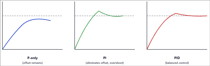
But proportional control has a weakness. It often leaves a small, constant error known as offset.

This happens because the controller always needs some error to generate an output. The system gets close to the setpoint, but not exactly there.

Integral Term (I) – Learning from the Past

The Integral term solves the offset problem. It looks at the error not just in the present, but over time.

• It adds up the error history, essentially remembering how long and how large the error has been.
• If a small error keeps occurring, the integral term grows until it pushes the system to eliminate it completely.
• Over time, this ensures the process reaches the exact setpoint.

But there is a catch. If the integral is set too strong, the system can overshoot. This means it goes past the setpoint and swings back, sometimes several times.

A related issue is integral windup, where the integral keeps building even when the actuator is already at maximum output.

Derivative Term (D) – Predicting the Future

The Derivative term acts like a predictor. It looks at how quickly the error is changing and estimates where it is headed.

• If the error is rising fast, the derivative provides a damping force to slow it down.
• This prevents overshoot and improves stability.
• It is especially useful in fast-moving processes, like speed control in motors.

However, derivative control is sensitive to noise. If the sensor signal is noisy, the derivative will amplify it, causing jerky outputs. For this reason, many industries use just PI control instead of full PID.

The Role of the PLC

In the past, engineers had to build dedicated hardware for PID control. Today, modern PLCs make it much easier. They come with built-in PID function blocks.

Integration

A PLC connects the sensor inputs (PV) and the actuators that carry out the control variable (CV).

Programming

In the PLC software, you simply insert a PID block, connect the PV and SP signals, and link the output to the device.

Tuning

The PLC stores the gain values for P, I, and D. You can adjust them directly through the interface.

This makes PID implementation more accessible. Even technicians who are not control theory experts can use PLC software to set up and tune loops.

Tuning Your PID Loop

Tuning is the art of adjusting the P, I, and D parameters until the system behaves well. The perfect settings depend on the process.

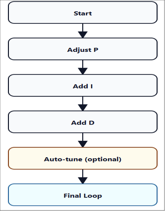
Start with P

Begin with only proportional control. Increase the gain until the system starts to oscillate, then reduce it to about half.

Add I

Introduce a small integral value. This removes steady-state error. Increase it slowly until the error disappears without causing big swings.

Add D (if necessary)

If your process reacts quickly or tends to overshoot, add a little derivative action for damping.

Auto-tune

Many modern PLCs have an auto-tune feature. The system runs a test, observes behavior, and automatically suggests PID values.

Good tuning balances speed, accuracy, and stability. Poor tuning causes overshoot, oscillations, or sluggish response.

Real-World Examples

Let’s look at where PID control in PLCs is actually used:

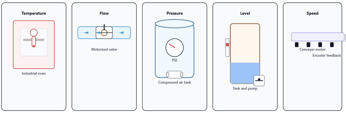
Temperature Control

In an industrial oven, the PLC reads temperature from a thermocouple (PV). It compares it to the setpoint (SP). The PID output adjusts gas or electric heaters. The result is precise, stable heating.

Flow Control

In pipelines, a PLC measures flow rate with a flow meter. The PID loop adjusts a motorized valve. This keeps the liquid flowing at the correct rate.

Pressure Control

In compressed air systems, a PID loop keeps tank pressure constant. It does this by controlling a compressor or a pressure valve.

Level Control

In tanks, the PLC monitors liquid level with a sensor. The PID loop controls pumps or valves to maintain the level.

Speed Control

Conveyor belts often require consistent speeds. A PID loop uses feedback from an encoder and adjusts the motor drive to hold steady speed.

Key Takeaways: PLC PID Control Explained Simply

PLC PID control is one of the most important tools in industrial automation. It is flexible, powerful, and surprisingly simple once you understand the basics.

Instead of crude ON/OFF control, a PID controller gives you three smart strategies — Proportional, Integral, and Derivative.

Together, they make the system respond not only to the present error, but also to past trends and future predictions.

A well-tuned PID loop can handle small drifts, sudden disturbances, and long-term stability.

Thanks to modern PLCs, implementing PID is easier than ever. Built-in blocks and auto-tuning make advanced control accessible even for non-specialists.

The payoff is huge: stable processes, better quality products, reduced wear on equipment, and more efficient energy use.

With a strong grasp of PID basics, you can start unlocking the full power of your automated systems.

FAQ: PLC PID Control Explained Simply

What does “PID” stand for in a PID controller?

PID stands for Proportional, Integral, and Derivative. These are the three control actions or terms that combine to determine the controller’s output based on how far, how long, and how fast the system error is changing.

What is a PID controller’s basic purpose?

A PID controller continuously compares a process variable (PV) with a desired setpoint (SP).

It then calculates an error (SP − PV), and uses the P, I, and D terms to adjust the output in order to reduce that error. The goal is to bring the process variable to the setpoint and keep it stable.

What does each term (P, I, D) do?

Proportional (P): Reacts to the current error. Larger error → larger correction. Helps reduce rise time but can leave a steady-state error.

Integral (I): Accumulates error over time. It addresses steady error or offset that P alone cannot eliminate.

Derivative (D): Looks at the rate at which error is changing. It acts to dampen or slow the controller’s response to prevent overshoot or oscillations. It’s like anticipating what might happen next.

Why is PID tuning important, and what are some common tuning methods?

Tuning means selecting or adjusting the gains (or time constants) of P, I, and D so the controlled process responds nicely (fast, stable, minimal overshoot, minimal steady error).

Without good tuning, the system might oscillate, respond too slowly, or constantly overshoot. 

Common tuning methods include: Manual tuning, by observing system behavior (e.g. increase P until borderline oscillation, then adjust I and D).

Auto-tuning, where the controller itself runs experiments to estimate good gains; Empirical rules like Ziegler-Nichols method.

What is “integral windup”, and how can it be prevented?

Integral windup occurs when the integral term builds up too much error — for example while the output is saturated (at its maximum or minimum limit) and cannot respond further.

When the constraint is removed, this “built up” integral can lead to overshoot or long settling times.

Prevention strategies include: Limiting or bounding the integral term; Using anti-windup logic (e.g. disabling integration when output is saturated or using back-calculation).

Can a PID controller have a simple ON/OFF output?

Yes, though that depends on application. The core PID algorithm usually produces an analog or continuously varying output.

But in some systems, that analog output is converted (via things like PWM or duty cycling) into ON/OFF switching to control physical devices (like heaters) that can’t respond continuously. 

What are the limitations of PID control?

Some limitations include: Sensitivity to noise, especially in the derivative term. Difficulties with non-linear systems or processes whose behavior changes with operating conditions.

Challenges in responding to large or sudden disturbances or changes in setpoint. If the system has long delays (dead time), PID can struggle; Potential overshoot or oscillations if tuning is not done properly. 

What is a “control loop” and what types are there?

A control loop refers to the cycle where the system measures a variable (PV), compares it with the desired value (SP), computes the error, uses a controller to adjust an actuator (CV), and affects the process, which feeds back into PV. This happens continuously.

Types include: Open loop, where no feedback is used — the controller doesn’t see the output; Closed loop, which is what PID control is — feedback is used to adjust continuously. 

How does the derivative term affect stability?

The derivative term adds damping. It helps reduce overshoot and smooth out fast changes.

That improves stability when things are changing rapidly. However, if derivative gain is too large, or if the sensor signal is noisy, it can cause erratic controller output or instability. 

What is “dead time” and how does it impact PID control?

Dead time (or delay) is the time lag between when the controller output changes and when its effect is first observed in the process variable. Long dead times make control harder because the system reacts slowly.

They can degrade performance, cause overshoot or oscillation, or make tuning more difficult. 

When might you use PI control instead of full PID?

PI (Proportional + Integral) control is often enough when the process is slower, or derivative action is not helpful (for example because of sensor noise, or small benefit versus complexity).

Many industrial applications omit the derivative term to simplify control and avoid amplifying noise. 

Dedicated PID devices vs. using a PLC for PID loops — which is better?

It depends on scale and complexity: Dedicated devices (stand-alone PID controllers) are good for simple, localized control (one loop, local HMI), fast deployment, less programming overhead.

PLCs are better when you need multiple loops, integration with other automation logic, data logging, supervising, HMI, alarms, etc.

They offer flexibility, communication, easier maintenance when multiple loops or complexity are involved.