controlcircuitry.com

All About Control Engineering

How to Tune a PID Controller

Posted on February 18, 2026 by Seki Hudson

PID stands for Proportional–Integral–Derivative, and remains the most widely used control algorithm in the global industry.

They are mainly used in industrial automation and robotics. Also, in areas such as power electronics and process control.

Their popularity comes from a good balance between simplicity and robustness. Plus, the performance they offer.

They possess a very simple structure. However, correctly tuning PID controllers can be a big challenge. Poor tuning may result in excessive overshoot.

It may cause slow response, oscillations, or even instability. On the other hand, a well-tuned PID controller can significantly improve system performance. It can reduce energy consumption and extend equipment life.

Fundamentals of PID control are explained in the present article. It provides practical, step-by-step guidance on how to tune a PID controller. Both classical and modern methods are covered.

Understanding the PID Controller

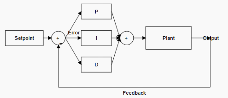
A PID controller generates a control signal based on the error (E). The error is between the desired setpoint and the actual measured output.

The output belongs to a system. The error signal is processed through three distinct terms.

These terms are proportional, integral, and derivative. Each term contributes differently to the controller’s behavior.

The proportional (P) term produces an output proportional to the current error. Increasing the proportional gain generally makes the system respond faster. Too much gain can cause oscillations or instability.

The integral (I) term accumulates past errors over time. This term is responsible for eliminating steady-state error.

Excessive integral action can lead to slow response. It can also cause oscillatory behavior known as integral windup.

The derivative (D) term predicts future error based on the rate of change. It improves damping and reduces overshoot. It is sensitive to noise and measurement disturbances.

Block diagram of a PID controller

Objectives of PID Tuning

Before tuning a PID controller, it is important to understand good performance. Good performance depends on the specific application. Common performance objectives include rise time and settling time.

They also include overshoot, steady-state error, and stability margin. Rise time refers to how quickly the system output reaches the desired setpoint.

Settling time measures how long the output takes to stabilize. Given a specific acceptable error band, this settling time must remain within it.

Most of the time, the output may exceed the setpoint. This phenomenon is known as overshoot. This happens before the system stabilizes.

Steady state error describes the final difference between the output and the setpoint. Stability ensures that the system does not oscillate indefinitely.

It also ensures the system does not diverge. Different applications prioritize different objectives. For example, motion control systems often prioritize fast response.

They also aim for low overshoot. Temperature control systems may tolerate slower responses. However, they require high stability and minimal oscillation.

Preparing the System for Tuning

Proper system preparation is the foundation of successful PID tuning. The first step is to understand the nature of the process.

This process is the one being controlled. Determine whether the system is fast or slow.

Also, check whether it is linear or nonlinear. Identify if it contains significant delays or dead time.

Verification of the proper calibration of sensors is a must. Make sure that noise is minimized. Actuators should operate within their limits.

In addition, safety constraints must be clearly defined. It is also important to disable integral and derivative action initially.

This is recommended when starting most tuning procedures. This simplifies the process.

It also reduces the risk of instability during early adjustments. If possible, perform tuning under normal operating conditions.

Tuning a controller at light load can cause problems. Unrealistic conditions can lead to poor performance. This poor performance appears during actual operation.

Manual PID Tuning Method

It is also called the Trial-and-Error method. Manual tuning is one of the most intuitive approaches.

It is also widely used in industrial environments. Although it may not produce mathematically optimal results, it is practical. It is effective for many systems.

The process usually starts by setting integral and derivative gains to zero. Increase the proportional gain gradually.

Continue until the system responds quickly. It should begin to oscillate slightly. At this point, reduce the proportional gain slightly.

This helps achieve a stable response. The response should have an acceptable speed. Next, introduce integral action to eliminate steady-state error. Increase the integral gain slowly, and continue until the steady-state error is removed.

This should occur within a reasonable time. Be cautious during this step. Too much integral gain can introduce oscillations. It can also cause sluggish behavior. Finally, add a derivative action to improve damping.

It also helps reduce overshoot. Increase the derivative gain gradually. Continue until oscillations are minimized.

The transient response should become smoother. Excessive derivative gain should be avoided since it is sensitive to noise.

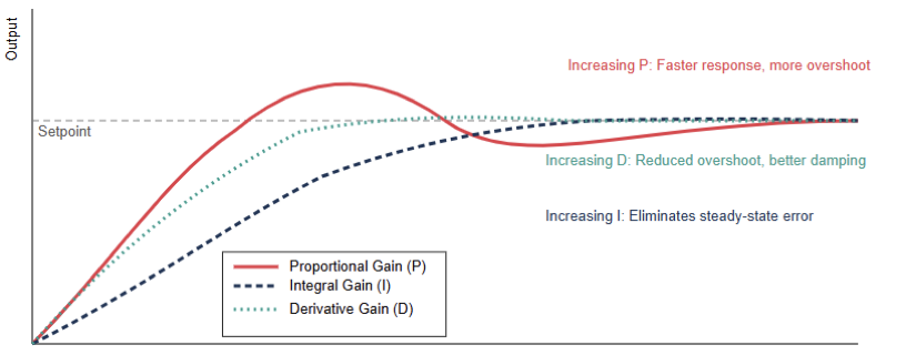
Step response plots showing the effect of increasing gains

Ziegler–Nichols Tuning Method

The Ziegler–Nichols method is one of the most well-known techniques. It is considered a classical tuning approach.

It provides systematic rules for selecting PID parameters. These rules are based on observed system behavior.

In the closed-loop Ziegler–Nichols method, integral and derivative gains are set to zero. The proportional gain is increased gradually.

This continues until the system reaches the ultimate gain. At this point, the system oscillates with constant amplitude.

The oscillation period is recorded. This value is known as the ultimate period. Using these two values, PID gains are calculated.

Predefined formulas are used. This method is simple and fast. However, it often results in aggressive tuning.

Significant overshoot is common. As a result, it is best suited for systems requiring fast response. Precision is less important in such cases.

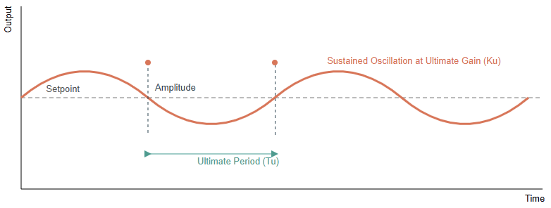
Sustained oscillation waveform used to identify key parameters

Cohen–Coon Tuning Method

The Cohen–Coon method is another classical approach. It is particularly useful for processes with significant dead time.

This method relies on an open-loop step response. The response belongs to the system being controlled.

By applying a step input, the output is observed. Key parameters are then estimated. These include process gain, time constant, and dead time. These parameters are used in empirical formulas. The formulas calculate PID gains.

Compared to Ziegler–Nichols, Cohen–Coon often provides better performance. This is especially true for slow processes.

These processes usually have delays; however, it requires a reliable open-loop test. This may not always be feasible, and it may also be unsafe in industrial systems.

Frequency-Domain and Model-Based Tuning

For applications requiring higher precision, advanced tuning methods are used. These include frequency-domain and model-based approaches. These methods rely on mathematical models. The models represent the system.

In frequency-domain tuning, tools such as Bode plots are used. Nyquist diagrams are also applied. These tools adjust PID gains.

The goal is to achieve desired gain and phase margins. This method provides strong insight into stability.

It also improves robustness. However, it requires control theory knowledge. Accurate system modeling is also required. Model-based tuning involves identifying a mathematical model.

The model represents the plant. PID parameters are computed using optimization techniques.

Many modern control software packages offer auto-tuning features. These features are based on these principles.

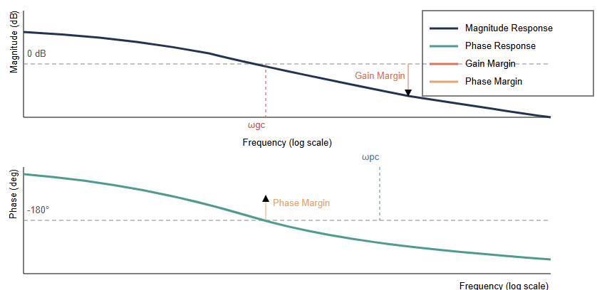
Bode plot illustrating gain margin and phase margin for PID tuning

Dealing with Integral Windup

Integral windup is a common problem in PID controllers. It is especially common when actuators saturate.

When the controller output is limited, problems arise. The integral term may continue to accumulate error. This leads to a large overshoot.

The overshoot occurs once the system returns to normal operation. Anti-windup techniques are used to mitigate this issue. Common methods include clamping the integral term.

Back-calculation is also used. Conditional integration is another method. Implementing anti-windup is essential for many systems.

This is especially true for systems with actuator limits. It is also important for frequent setpoint changes.

Effective PID Tuning: Practical Tips

Applying practical guidelines can improve tuning outcomes. Always make small changes to gain. Then observe the system response.

Document parameter changes and results, as it helps avoid confusion. Use filters on the derivative term.

This reduces noise sensitivity. It is also important to consider sampling time. This applies to digital PID controllers. An inappropriate sampling period can degrade performance.

It can also cause instability. Finally, remember that tuning is often iterative. Real-world systems may require periodic retuning. This is due to wear, load changes, or environmental variations.

Auto-Tuning and AI

Currently, many high-end PLCs feature Auto Tune buttons. PLCs are Programmable Logic Controllers that use relay oscillation techniques. The goal is to automatically determine optimal parameters.

Furthermore, AI-based tuning is emerging. These systems monitor the machine continuously.

They operate restlessly, and if a bearing starts to wear, adjustments are made. If a load changes, compensation is applied.

The AI silently adjusts the PID values. This process compensates for system changes. This approach is known as adaptive control. The result is peak operational efficiency with reduced human intervention.

PID Tuning: Common Pitfalls to Avoid

Common issues during the tuning of a PID controller:

Over-tuning: Trying to make a slow system behave like a fast one. A large oven should not act like a motor. This approach only leads to instability.
Ignoring noise: Derivative action amplifies noise. If the sensor signal is not filtered, problems occur. The derivative gain can vibrate actuators excessively.
Loop interaction: In complex factories, one PID loop may fight another. Always tune the innermost loop first. The most critical loop should be prioritized.

Conclusion

The present article covered the fundamentals of PID control. It provided practical guidance for tuning PID controllers.

Both classical and modern methods were discussed. Tuning a PID controller is both an art and a science.

The underlying principles are well established. Real-world systems introduce uncertainties.

These uncertainties require practical judgment and experience. By understanding each PID term, engineers improve results.

Clear performance objectives must be defined. Appropriate tuning methods should be applied.

This leads to stable and efficient control. Manual tuning has its place, in which a classical method like Ziegler–Nichols are useful.

Modern model-based techniques are also valuable. With careful preparation and systematic adjustment, PID controllers deliver reliable control. They provide high-quality performance across many applications.

PID Controllers Made Simple

FAQ: How to Tune a PID Controller

What does “tuning a PID controller” mean?

Tuning a PID controller means choosing appropriate values for the proportional (P), integral (I), and derivative (D) gains so the controlled system responds well to changes in setpoint and disturbances, balancing speed, stability, and overshoot.

Why is PID tuning important?

Incorrect tuning can lead to oscillations, slow response, overshoot, or even instability. Proper tuning ensures predictable, efficient control and reduces wear on equipment.

What are the common methods for tuning a PID controller?

There are several methods, including manual trial-and-error, Ziegler–Nichols method, Cohen–Coon method, and software-based model tuning tools like MATLAB’s PID Tuner, which use response data to compute gains.

What is the Ziegler–Nichols tuning method?

It’s a heuristic tuning approach where you set I and D to zero, increase P until sustained oscillation occurs, record the gain (Ku) and period (Tu), and then apply formulas to calculate P, I, and D gains.

Should I start tuning with all gains at zero?

Yes. A common practical approach is to start with I and D at zero, increase P until the output responds and, if necessary, oscillates lightly, then bring in I to eliminate steady-state error and D to reduce overshoot.

How Does a Limit Switch Work?

Posted on February 18, 2026 by Seki Hudson

Reliability of industrial automation still rests on the shoulders of the humble limit switch. In recent years, there has been a rise in advanced proximity and laser sensors.

Nevertheless, the limit switch remains the most trusted device for physical position verification

They ensure safety, accuracy, and repeatability in machines. These machines range from conveyor systems to CNC equipment.

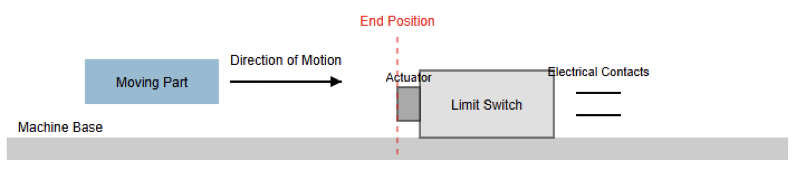
A limit switch provides a clear, deterministic signal. It indicates that a moving part has reached a predefined position.

Unlike noncontact sensors, limit switches rely on physical interaction. This makes them robust even in harsh environments. It also makes them more predictable. Understanding how a limit switch works is essential for engineers.

This article details the construction and operating principle. It also explains the applications and advantages of limit switches. These are relevant in modern industrial systems.

Understanding Limit Switch

A limit switch is an electromechanical device. It is designed to detect the presence or position of an object.

This detection occurs by means of physical contact. When a machine component reaches a specific point, it actuates the switch.

This component may be a cam, lever, or moving carriage. The actuation is mechanical in nature. This action changes the state of the electrical contacts inside the switch.

It sends a signal to a control system. This system may be a PLC, relay logic circuit, or motor controller.

Limit switches are commonly used to:

Stop motion at the end of travel
Confirm position or alignment
Prevent mechanical over-travel
Initiate a sequence of operations

Their simplicity makes them easy to apply. Their reliability supports long-term operation. Their clear ON/OFF output simplifies control logic. These characteristics make them critical for many industrial uses.

Main Components of a Limit Switch

Limit switches come in many shapes and sizes. However, their internal structure is consistent.

Each component plays a specific role. This role involves converting mechanical motion into an electrical signal.

Actuator (Operating Head)

The actuator is the external part of the switch. It makes contact with the moving object. Common actuator types include:

Plunger
Roller lever
Whisker (spring rod)
Rotary cam lever

The choice of actuator depends on the motion type. It also depends on speed, accuracy, and durability requirements.

Mechanical Transmission Mechanism

Inside the switch, the actuator connects to a mechanical linkage. It may also connect to a spring-loaded mechanism.

This mechanism ensures that a small external movement is effective. It produces a decisive internal action.

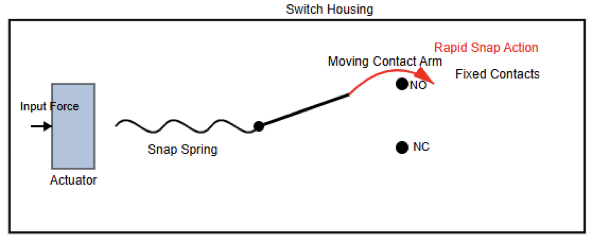
Many limit switches use a snap-action mechanism. This mechanism guarantees fast and consistent contact switching.

Electrical Contacts

The contacts are the electrical heart of the limit switch. They can be:

Normally Open (NO)
Normally Closed (NC)
Changeover (SPDT)

The contact configuration determines circuit behavior. It defines how the control system responds. This response occurs when the switch is actuated.

Housing and Sealing

The housing protects internal components. It shields them from dust and moisture. Also, against oil as well as mechanical damage.

Industrial-grade limit switches often meet IP65 standards. Many also meet IP67 or higher protection ratings.

The following figure indicates a diagram of an exploded view of a limit switch showing actuator, spring mechanism, contacts, and housing.

Operating Principle of a Limit Switch

The working principle of a limit switch is mechanical. It is based on displacement leading to electrical switching. This process can be broken down into stages. These stages are clear and repeatable.

When a moving machine part approaches the limit switch, it makes contact. The contact occurs with the actuator.

As the actuator moves, it transfers force inward. This force reaches the internal mechanical mechanism.

Once a predefined travel distance is reached, switching occurs. A force threshold may also trigger this event. The mechanism then produces a snap action.

This snap action changes the state of the electrical contacts. It either opens or closes the circuit.

When the object moves away, the actuator returns. It moves back to its original position under spring force.

The contacts then revert to their normal state. This action is repeatable over time. It allows consistent position feedback. This feedback remains accurate over millions of cycles.

Normally Open and Normally Closed Operation

Understanding contact behavior is essential. It is especially important when designing control circuits.

A Normally Open (NO) contact remains open initially. This occurs when the switch is not actuated. When the actuator is pressed, the contact closes.

This allows current to flow. NO contacts are commonly used for signaling. They are also used for event detection.

On the other hand, a Normally Closed (NC) contact remains closed initially. This occurs when the switch is not actuated.

When the actuator is pressed, the contact opens and interrupts the circuit. NC contacts are widely used in safety circuits. A broken wire results in a safe condition. A failed switch also produces an open circuit.

Many industrial limit switches provide both contact types. They include NO and NC contacts. This offers flexibility in control logic design.

Snap-Action Mechanism

One defining feature of a quality limit switch is the snap-action mechanism. Instead of slow contact movement, it ensures rapid switching. Contacts change state quickly. This occurs once the actuation point is reached.

This behavior provides several advantages:

Reduced electrical arcing
Consistent switching point
Improved contact life
Reliable operation at low voltages and currents

Snap-action behavior is especially important in control circuits. It supports precise timing requirements.

It also maintains signal integrity. The next figure indicates a diagram of an internal snap-action mechanism illustrating rapid contact switching.

Electrical Integration in Control Systems

Limit switches are typically wired into control circuits. These circuits use low-voltage signals. Common values include 24 V DC or 120 V AC. The choice depends on regional standards.

Application requirements also influence the selection. In modern systems, switches connect to PLC digital inputs.

When the limit switch changes state, the PLC detects it. The PLC sees the input transition and then executes programmed logic, such as:

Stopping a motor
Reversing direction
Triggering an alarm
Initiating the next step in a sequence

In relay-based systems, limit switches control contactors directly. They may also control auxiliary relays.

This approach provides reliable automation logic. It is also straightforward to implement.

Applications of Limit Switches

Limit switches are used across many industries. This is due to their robustness and simplicity. In material handling systems, they detect conveyor endpoints.

They prevent belt overrun conditions. In machine tools, they establish reference positions.

They also prevent axis collisions. Elevators and hoists rely on limit switches. These are used for travel limits and safety interlocks.

In packaging machinery, limit switches ensure proper positioning. They also maintain synchronization of moving parts.

Their ability to function reliably is significant. They work in dusty environments. They also operate in oily and high-vibration conditions. This makes them suitable for industrial use.

Advantages of Using Limit Switches

Limit switches offer several practical advantages. These advantages exceed those of some sensing technologies.

They provide positive mechanical feedback. This ensures the detected position is physically reached.

Their operation is immune to electrical noise. It is also unaffected by optical interference. They are cost-effective solutions, and installation is straightforward. Troubleshooting is simple, and they can operate in extreme temperatures.

They also function in harsh environments. Electronic sensors may fail under these conditions. For safety-related functions, limit switches are preferred.

Their fail-safe wiring options build trust. They are widely accepted in industrial standards. Regulations also recognize their reliability.

Limit Switches vs Non-Contact Sensors

While limit switches are highly reliable, they are not universal. They are not always the best choice. On the other hand, non-contact sensors offer certain advantages.

These include inductive, capacitive, and photoelectric sensors. Such sensors work well in high-speed applications. They also eliminate physical wear.

However, limit switches excel in specific cases:

Physical confirmation of position is required
The environment is harsh
The application demands simplicity and reliability
Safety circuits are involved

In many systems, both sensor types are used. Limit switches and non-contact sensors complement each other. This balances precision and robustness.

Key Selection Factors

When selecting a switch, consider key variables:

Environmental Sealing: Does it require an IP67 rating? This is critical for washdown environments.
Contact Rating: Will it trigger a low-power PLC signal? Or will it control a high-power motor starter?
Operating Force: How heavy is the target? A glass bottle differs from a steel beam.
Frequency of Operation: How many times per minute will it actuate? High-speed lines require long-life variants.

Common Failure Modes and Maintenance

Although durable, limit switches can fail. They are not immune to wear. Common issues include mechanical wear of the actuator.

Contact degradation may occur due to arcing. Environmental damage can result from moisture or contaminants.

Preventive maintenance includes:

Regular inspection of actuator alignment
Checking contact operation and wiring integrity
Ensuring proper sealing and mounting
Replacing switches after their rated mechanical life

Proper installation is critical. Regular maintenance is equally important. Together, they significantly extend operational life.

Conclusion

This article addressed the working principles of limit switches. It also covered construction and practical applications.

Limit switches are fundamental components in automation. They provide reliable and precise position detection.

This is achieved through simple electromechanical principles. By converting physical motion into an electrical signal, they enable safety.

They also support accurate control and effective sequencing. Their snap-action mechanisms improve reliability.

Flexible contact configurations add versatility. Rugged construction supports demanding applications.

Modern non-contact sensors offer advanced capabilities. However, the limit switch remains irreplaceable.

This is especially true in safety-critical environments. Harsh conditions further reinforce their value.

A solid understanding of limit switch operation is essential. It allows engineers and technicians to design reliable systems. It also supports safe and efficient industrial operations.

Frequently Asked Questions

What is a limit switch?

A limit switch is an electromechanical device that detects the presence, absence, or position of a moving part. It changes the state of an electrical circuit when it is actuated by a mechanical force.

How does a limit switch operate?

When a moving machine part contacts the actuator (like a plunger, lever, or roller), it pushes the internal mechanism.

At a certain point, this movement triggers internal contacts to open or close, changing the electrical circuit state. This is often done via a snap-action mechanism for fast and reliable switching.

What triggers a limit switch?

A limit switch is typically triggered by physical contact with a mechanical movement, such as a conveyor item, robot arm, or machine carriage. Some designs also activate through rotational movement or cam engagement.

What are the main contact types in a limit switch?

Limit switch contacts can be Normally Open (NO) or Normally Closed (NC).

NO contacts close when the actuator is pressed.
NC contacts open when actuated.

Why do many limit switches use snap-action mechanisms?

Snap-action mechanisms ensure the contacts switch state quickly and cleanly, minimizing electrical arcing and contact bounce. This increases the reliability and lifespan of the switch.

Types of Encoders

Posted on February 18, 2026 by Seki Hudson

In current motion control within automation systems, encoders play a critical role. They are essential devices in modern automation and control systems. They convert mechanical motion into electrical signals.

These signals are then interpreted by controllers, drives, or monitoring systems. Encoders are widely used in industrial machinery and robotics.

They are also found in CNC machines, elevators, and renewable energy systems.

Accurate position and speed feedback is critical in these applications. Different encoder types exist to meet different accuracy and speed requirements. Also, to meet environmental requirements, which are essential.

There are different types of encoders. Understanding encoder types is important for choosing the correct device for a specific task.

This article explains the main types of encoders by comparing their working principles, advantages, and applications.

Understanding Encoder

An encoder is a feedback sensor that detects motion. Motion can be rotational or linear. The encoder converts this motion into digital or analog signals.

These signals represent position, speed, direction, or distance. Controllers use this data for precise control.

Encoders improve accuracy and repeatability. They are critical in closed-loop control systems.

Classification of Encoders

Encoders can be classified in several ways. The most common classifications are based on motion type and output type. Each classification addresses a specific application need.

The main categories are rotational and linear encoders. Another major division is incremental and absolute encoders. Encoders can also be classified by sensing technology.

Rotational Encoders

Rotational encoders measure angular position or speed. They are mounted on rotating shafts.

They are common in motors and gear systems. Rotational encoders are used in conveyors, servo motors, and pumps.

Optical Rotational Encoders

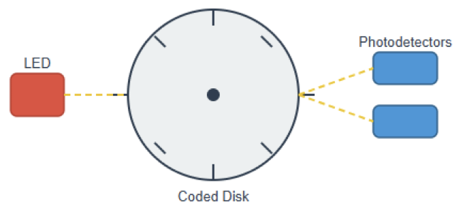
Optical encoders use light for sensing. A coded disk is attached to the shaft, and a light source shines through the disk. Photodetectors receive the light. Slots or patterns on the disk interrupt the light.

The output depends on disk rotation. High resolution is possible. Optical encoders are very accurate. They are sensitive to dust and moisture.

Magnetic Rotational Encoders

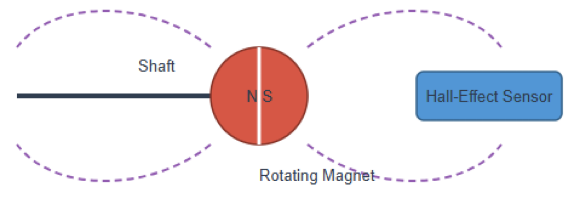
Magnetic encoders use magnetic fields. A magnet is attached to the shaft, and a magnetic sensor detects field changes. Hall-effect or magneto-resistive sensors are common.

These encoders are robust due to their tolerance to dust and vibration. Resolution is lower than optical types. They are ideal for harsh environments.

Linear Encoders

Linear encoders measure straight-line motion. They are used in machine tools and positioning systems. They provide direct measurement of displacement.

Optical Linear Encoders

Optical linear encoders use a scale and a read head. The scale has fine markings. Light passes through the scale, and the read head detects movement.

They provide very high accuracy. CNC machines are the common use. To take advantage of them, clean environments are required.

Magnetic Linear Encoders

Magnetic linear encoders use a magnetic strip. A sensor reads magnetic transitions. These kinds of encoders are less sensitive to contamination.

They are easier to install, and their accuracy is moderate. They are common in industrial automation.

Incremental Encoders

These encoders rely on pulse generation. This means incremental encoders generate pulses when motion occurs.

They do not store absolute position. Position is determined by counting pulses. If power is lost, the position is lost.

Incremental encoders are simple. They are cost-effective. This is why they are widely used in speed measurement.

Working Principle

When the shaft rotates, pulses are generated. Each pulse represents a fixed movement. Two output channels are usually provided.

These are called A and B, and they are phase-shifted. The phase shift indicates direction. A third channel may exist. It is called the index or Z channel and provides a reference position.

Advantages and Limitations

They are simple to use. They have high-resolution options and are affordable. They are suitable for speed control.

Position is lost on power failure, so homing is required after restart. External counters are needed.

Absolute Encoders

Absolute encoders provide a unique position value. Each position has a distinct code. Position is retained after power loss.

In this case, no homing is required. Absolute encoders are used where safety and accuracy are critical. They are common in robotics and cranes.

Single-Turn Absolute Encoders

Single-turn encoders measure position within one rotation. The output resets after one revolution.

Each angular position has a unique code. They are used in valve positioning. They are very common in servo systems.

Multi-Turn Absolute Encoders

Multi-turn encoders track multiple rotations. They store the rotation count internally. Mechanical gears or electronic counters are used, and they provide full position information. The main use is in elevators and wind turbines.

Encoder Output Types

Encoders differ in output format. Output type affects compatibility and noise immunity. Encoder output types describe the electrical signal format, with the most common being Open Collector.

Also, Push-Pull (Totem Pole/HTL)and Differential Line Driver (TTL). Each is suited for different applications and noise levels.

They convert position/motion into digital signals like pulses (incremental) or unique codes (absolute) for PLCs.

It may also include microcontrollers. Voltage levels and current sourcing/ or sinking capabilities are the main keys for their differentiation.

Digital Encoders

Digital encoders produce pulses or binary data. Incremental and absolute encoders fall into this category.

The digital outputs are always robust. Plus, they are really easy to interface with PLCs. Common interfaces include TTL, HTL, and RS-422.

Analog Encoders

Analog encoders produce continuous signals. Output may be voltage or current. Examples include 0–10 V or 4–20 mA. They provide smooth position feedback. Their resolution is lower, and they are sensitive to noise.

Contact and Non-Contact Encoders

Encoders can also be classified by sensing contact.

Contact Encoders

Contact encoders use physical contact. Potentiometer-based encoders are examples. A wiper moves along a resistive track. They are simple and inexpensive. Wear occurs over time, and accuracy degrades.

Non-Contact Encoders

Non-contact encoders use optical or magnetic sensing. There is no mechanical wear. Lifespan is longer, and accuracy is higher. Most modern encoders are non-contact types.

Capacitive Encoders

Capacitive encoders detect changes in capacitance. A patterned scale is used. Movement changes the electric field.

They offer good resolution and are immune to magnetic fields. They are sensitive to humidity and contamination. Commonly, they are used in precision instruments.

Inductive Encoders

Inductive encoders use electromagnetic induction. A conductive scale interacts with coils. Position is detected through signal changes.

They are extremely robust. Since they tolerate oil and dirt, the accuracy is moderate. They are popular in heavy industrial environments.

Resolver as a Special Encoder Type

Resolvers are analog rotary position sensors. They resemble rotary transformers. Output signals are sine and cosine waves.

Resolvers are very robust, and they operate in extreme temperatures. In this type, signal processing is complex. They are used in aerospace and military systems.

Comparison of Encoder Types

Different encoder types suit different needs. Optical encoders offer high precision. Magnetic encoders offer durability.

While incremental encoders are simple and fast. On the other hand, absolute encoders provide safety and reliability.

Also, linear encoders provide direct position measurement. Plus, rotational encoders measure angular motion. The environment often dictates the choice.

Applications of Encoders

Encoders contain a vast number of applications. A few are briefly explained below

· Robotics: Encoders are used for precise joint position and motion control.

· CNC machines: They provide accurate axis positioning and feedback.

· Conveyor systems: Encoders are applied for speed monitoring and control.

· Elevators: Absolute encoders are relied upon for safe and accurate position detection.

· Renewable energy systems: Encoders are used for blade and pitch positioning.

· Packaging machines: Precise synchronization depends on encoder feedback.

Selecting the Right Encoder

When choosing an encoder in the market, engineers must weigh several competing factors. One key factor is resolution requirements.

This defines how many counts per revolution are needed for accurate measurement. A precision lathe may require around 10,000 pulses per revolution.

A simple garage door system may function well with only 100 pulses. Mounting space is another important consideration. Some applications have very limited physical space.

This is common in small drone motors and compact actuators. In such cases, magnetic or capacitive kit encoders are preferred. They offer a very low profile and flexible integration.

Safety integrity level is also critical. Currently, safety-rated encoders are mandatory for human-collaborative robots. These encoders include redundant internal circuits.

The redundancy prevents runaway motion if one internal component fails. This greatly improves system safety and reliability.

Conclusion

This article dealt with the main types of encoders. It explained their working principles, advantages, and applications. It also addressed the selection criteria. Encoders are vital components in motion control systems.

Encoders are no longer just sensors; they are the fundamental data source for the physical world.

They provide accurate feedback for position, speed, and direction. Many encoder types exist. Each type serves a specific purpose.

For instance, incremental encoders are simple and economical. Absolute encoders provide reliable position data.

Optical encoders offer high precision. Magnetic and inductive encoders provide durability.

Linear and rotational encoders address different motion types. Proper encoder selection must be taken into account.

This is because it improves system performance and reliability. Efficient and safe automation systems can be designed if engineers understand encoder types.

Temperature Transmitter Calibration

Posted on February 18, 2026 by Seki Hudson

Temperature transmitters are critical instruments in industrial measurement and control systems.

They convert temperature signals into standardized outputs. These outputs are commonly 4–20 mA or digital signals.

Accurate temperature measurement is essential for safety. Also, for quality and efficiency. Over time, transmitters can drift.

Environmental conditions and aging cause errors. To detect and correct these errors, the process of calibration comes into action.

Correct calibration provides measurement reliability and regulatory compliance. This article explains temperature transmitter calibration in detail.

It covers principles, equipment, and procedures. In addition, it details the errors and best practices.

A Temperature Transmitter

A temperature transmitter is an electronic device. It acquires an input signal from a temperature sensor.

RTDs or thermocouples are the typical sensors used. The transmitter converts this signal into a standardized output.

The output is sent to a controller or monitoring system. This allows temperature values to be read remotely. It also improves noise immunity.

Transmitters are used in process industries. Examples include oil and gas, power plants, and food processing.

Basic Calibration Concepts

Calibration compares an instrument to a reference. The reference must be more accurate. The difference between the two is the error. Calibration may include adjustment.

Verification-only calibration checks accuracy without adjustment. Traceability is essential. This means the reference is linked to national standards. Also, uncertainty must be known. Plus, calibration results should be documented.

Why Calibration Is Necessary

Calibration ensures measurement accuracy. No instrument remains accurate forever. Temperature transmitters drift due to component aging.

Vibration and thermal cycling also affect performance. Incorrect temperature readings can cause product defects.

They can also create safety risks. Regulatory standards often require periodic calibration. Calibration verifies that the transmitter output matches the true temperature. It also allows adjustment when errors exceed tolerance.

Temperature Sensors Used with Transmitters

Temperature transmitters work with different sensors. RTDs are common in industrial applications.

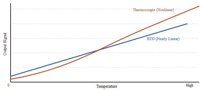
They offer high accuracy and stability. Platinum RTDs like Pt100 are widely used. On the other hand, the thermocouples are also popular.

They cover a wide temperature range. Plus, they are rugged and simple. Each sensor type affects calibration. The transmitter must be calibrated for the correct sensor.

Calibration Standards and References

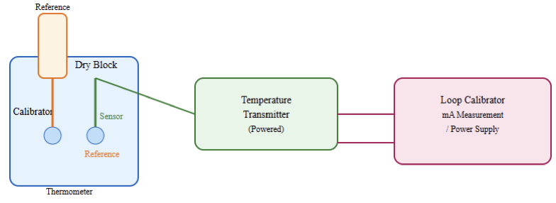
Accurate calibration requires reliable references. Dry block calibrators are widely used. They provide stable temperature sources.

In addition, liquid baths are used for high-accuracy work. Reference thermometers measure the true temperature.

These may be standard RTDs or precision thermometers. Electrical simulators can also be used. They simulate sensor signals directly. This is common for bench calibration.

What is temperature transmitter calibration?

Calibration is the process of comparing the performance of a device against a known standard. For a temperature transmitter, this involves two distinct steps. First, we test the sensing element, such as an RTD or thermocouple.

Second, we test the transmitter’s ability to convert that sensor data into a standardized output. Currently, most technicians perform a loop calibration.

This tests the entire measurement chain. Usually, from the heat source to the control room display.

If both the transmitter and the standard read 100°C, the system is within tolerance. Any deviation requires adjustment to align the transmitter with the reference.

Types of Temperature Transmitter Calibration

Calibration can be done in different ways. In-situ calibration is performed in the field. The transmitter remains installed.

While bench calibration is done in a workshop. Loop calibration checks the entire measurement loop.

Point calibration checks specific temperatures. And multi-point calibration checks linearity. Two-point calibration is common. It is used to check zero and span.

Calibration Range and Span

The calibration range is the temperature interval tested. The span is the difference between the upper and lower limits. Calibration should cover the operating range. Testing outside the range is not useful.

Zero corresponds to the lower range value. Span corresponds to the upper range value. Errors at zero and span affect the entire range.

Common Calibration Equipment

To perform a professional calibration, specialized equipment is required. A temperature standard, such as a dry-block calibrator or a stirred liquid bath, is used to provide a stable and known temperature reference.

A reference thermometer is also necessary, typically a high-accuracy probe like a Platinum Resistance Thermometer, which serves as the master measurement for comparison.

In addition, a process calibrator is used to measure the 4–20 mA output signal from the transmitter.

For smart transmitters, a HART or Fieldbus communicator is required to adjust internal parameters and complete the calibration process accurately.

Calibration Procedure Overview

Calibration follows a structured process. First, review transmitter specifications. Check the sensor type and range.

Inspect the transmitter physically. Apply power and allow warm-up. Apply known temperature points.

Measure the output at each point. Compare results with expected values. Then, adjust if necessary. Repeat measurements after adjustment and document all results.

Step-by-Step Calibration Example

A Pt100 temperature transmitter operates over a range of 0 to 100 °C and provides a 4–20 mA output signal.

Insert the sensor into a dry block. Set the dry block to 0 °C and allow stabilization. Measure the output current.

The latter should be 4 mA. Record the value. Increase the temperature to 100 °C. Allo